Generating input grids#
The simulation mesh describes the number and topology of grid points, the spacing between them, and the coordinate system. For many problems, a simple mesh can be created using options.
[mesh]
nx = 260  # X grid size
ny = 256  # Y grid size

dx = 0.1  # X mesh spacing
dy = 0.1  # Y mesh spacing
The above options will create a \(256\times 256\) mesh in X and Y, assuming there are 2 guard cells in X direction. The Z resolution can be specified with MZ. The mesh spacing is \(0.1\) in both directions. By default the coordinate system is Cartesian (metric tensor is the identity matrix), but this can be changed by specifying the metric tensor components.
Integer quantities such as nx can be numbers (like “260”), or
expressions (like “256 + 2*MXG”).
A common use is to make x and z dimensions have the same
number of points, when x has mxg boundary cells on each
boundary but z does not (since it is usually periodic):
[mesh]
nx = nz + 2*mxg  # X grid size
nz = 256         # Z grid size
mxg = 2
Note that the order of the defintion within a section isn’t important, variables can be used before they are defined. All variables are first read, and only processed if they are used.
Expressions are always calculated in floating point; When expressions
are used to set integer quantities (such as the number of grid
points), the expressions are calculated in floating point and then
converted to an integer. The conversion is done by rounding to the
nearest integer, but throws an error if the floating point value is
not within 1e-3 of an integer. This is to minimise unexpected
behaviour. If you want to round any result to the nearest integer, use
the round function:
[mesh]
nx = 256.4   # Error!
nx = round(256.4) # ok
Real (floating-point) values can also be expressions, allowing quite
complicated analytic inputs. For example in the example test-griddata:
# Screw pinch

rwidth = 0.4

Rxy = 0.1 + rwidth*x  # Radius from axis     [m]
L   = 10              # Length of the device [m]

dy = L/ny
hthe = 1.0

Zxy = L * y / (2*pi)

Bpxy = 1.0      # Axial field [T]
Btxy = 0.1*Rxy  # Azimuthal field [T]
Bxy = sqrt(Btxy^2 + Bpxy^2)

dr = rwidth / nx
dx = dr * Bpxy * Rxy
These expressions use the same mechanism as used for variable
initialisation (Expressions): x is a variable from
\(0\) to \(1\) in the domain which is uniform in index space;
y and z go from \(0\) to \(2\pi\). As with variable
initialisation, common trigonometric and mathematical functions can be
used. In the above example, some variables depend on each other, for
example dy depends on L and ny. The order in which these
variables are defined doesn’t matter, so L could be defined below
dy, but circular dependencies are not allowed (by default; see
section Recursive functions). If the variables are defined
in the same section (as dy and L) or a parent section, then no
section prefix is required. To refer to a variable in a different
section, prefix the variable with the section name, for example,
section:variable or mesh:dx.
More complex meshes can be created by supplying an input grid file to describe the grid points, geometry, and starting profiles. Currently BOUT++ supports NetCDF format binary files. During startup, BOUT++ looks in the grid file for the following variables. If any are not found, a warning will be printed and the default values used.
X and Y grid sizes (integers)
nxandnyREQUIREDDifferencing quantities in 2D/3D arrays
dx(nx,ny[,nz]),dy(nx,ny[,nz])anddz(nx,ny[,nz]). If these are not found they will be set to 1. To allow variation inzdirection, BOUT++ has to be configured-DBOUT_ENABLE_METRIC_3D, otherwise 2D fields are used for the metric fields. Note that prior to BOUT++ version 5dzwas a constant.Diagonal terms of the metric tensor \(g^{ij}\)
g11(nx,ny[,nz]),g22(nx,ny[,nz]), andg33(nx,ny[,nz]). If not found, these will be set to 1.Off-diagonal metric tensor \(g^{ij}\) elements
g12(nx,ny[,nz]),g13(nx,ny[,nz]), andg23(nx,ny[,nz]). If not found, these will be set to 0.Z shift for interpolation between field-aligned coordinates and non-aligned coordinates (see Field-aligned coordinates). Parallel differential operators are calculated using a shift to field-aligned values when
paralleltransform:type = shifted(orshiftedinterp). The shifts must be provided in the gridfile in a fieldzShift(nx,ny). If not found,zShiftis set to zero.
The remaining quantities determine the topology of the grid. These are based on tokamak single/double-null configurations, but can be adapted to many other situations.
Separatrix locations
ixseps1, andixseps2If neither is given, both are set to nx (i.e. all points in closed “core” region). If onlyixseps1is found,ixseps2is set to nx, and if only ixseps2 is found, ixseps1 is set to -1.Branch-cut locations
jyseps1_1,jyseps1_2,jyseps2_1, andjyseps2_2Twist-shift matching condition
ShiftAngle[nx]for field aligned coordinates. This is applied in the “core” region between indicesjyseps2_2, andjyseps1_1 + 1, if eitherTwistShift = Trueenabled in the options file or in general theTwistShiftflag inmesh/impls/bout/boutmesh.hxxis enabled by other means. BOUT++ automatically reads the twist shifts in the gridfile if the shifts are stored in a field ShiftAngle[nx]; ShiftAngle must be given in the gridfile or grid-options ifTwistShift = True.
The only quantities which are required are the sizes of the grid. If these are the only quantities specified, then the coordinates revert to Cartesian.
This section describes how to generate inputs for tokamak equilibria. If you’re not interested in tokamaks then you can skip to the next section.
The directory tokamak_grids contains code to generate input grid
files for tokamaks. These can be used by, for example, the 2fluid and
highbeta_reduced modules.
BOUT++ Topology#
Basic#
BOUT++ is designed to work in a variety of tokamak and non-tokamak
geometries, from simple slabs to disconnected double-null
configurations. In order to handle tokamak geometry BOUT++ contains an
internal topology which is built from six regions determined by four
branch-cut locations and two separatrix locations (ixseps1 and
ixseps2). There are some limitations on these regions that we will
discuss below, and some regions may be empty, all of which enables
BOUT++ to describe effectively seven types of topology:
“core”: this type of topology can describe the closed field line regions inside the separatrix of tokamaks or other devices, or idealised geometries like periodic slabs;
“SOL”: these can describe the open field line regions of the scrape-off layer (SOL) outside the separatrix of a tokamak, or linear devices with a target plate at either end;
“limiter”: these topologies have an open field line region and a region where field lines hit a boundary, without an X-point;
“X-point”: these topologies have four separate legs with their own boundaries, and no closed field line region;
“single null”: this type of topology has one X-point with two separate legs, closed and an open field line regions, and a single separatrix;
“connected double null”: these topologies have two X-points with two separate legs each, closed and open field line regions and a single separatrix that connects both X-points;
“disconnected double null”: finally, these are similar to connected double null geometries except that they have two separatrices that do not connect the two X-points. These come in “lower” and “upper” flavours, depending on which X-point is adjacent to the closed field line region.
The six regions that form the building blocks of these topologies are:
four separate “leg” regions that have a boundary in the
ydirection;two “core” regions that do not have boundaries in
y.
Each of these regions may have additional boundaries in the x
direction. The separate regions are illustrated in
Fig. 5: the grey dashed lines show the
region partitions, with the sections labelled 1, 2, and 3 forming one
leg; 4, 5, and 6 forming one core region, and so on. The internal names
for these separate regions use “inner” and “outer” in reference to the
major radius – that is, “inner” regions correspond to the left-hand
side of Fig. 5 and “outer” regions to the
right-hand side.
Two important limitations for BOUT++ grids are that a single processor can only belong to one region, and that there must be the same number of points on each processor. The first limitation means that certain topologies require a minimum number of processors. For example, a disconnected double null configuration uses all six regions – therefore the minimum number of processors able to describe this in BOUT++ is six. Having equal numbers of points on each processor can put some restrictions on the resolution of simulations.
The two separatrix locations are ixseps1 and ixseps2, these are
the global indices in the x domain where the first and second
separatrices are located. These values are set either in the grid file
or in BOUT.inp. Fig. 5 shows
schematically how ixseps is used.
If ixseps1 == ixseps2 then there is a single separatrix representing
the boundary between the core region and the SOL region and the grid is
a connected double null configuration. If ixseps1 > ixseps2 then
there are two separatrices and the inner separatrix is ixseps2 so
the tokamak is an upper double null. If ixseps1 < ixseps2 then there
are two separatrices and the inner separatrix is ixseps1 so the
tokamak is a lower double null.
In other words: Let us for illustrative purposes say that ixseps1 >
ixseps2 (see Fig. 5). Let us say that we
have a field f(x,y,z) with a global x-index which includes ghost
points. f(x <= ixseps1, y, z)) will then be periodic in the
y-direction, f(ixspes1 < x <= ixseps2, y, z)) will have boundary
condition in the y-direction set by the lowermost ydown and
yup. If f(ixspes2 < x, y, z)) the boundary condition in the
y-direction will be set by the uppermost ydown and yup. As
for now, there is no difference between the two sets of upper and lower
ydown and yup boundary conditions (unless manually specified,
see Custom boundary conditions).
The four branch cut locations, jyseps1_1, jyseps1_2,
jyseps2_1, and jyseps2_2, split the y domain into logical
regions defining the SOL, the PFR (private flux region) and the core of
the tokamak. This is illustrated also in
Fig. 5. If jyseps1_2 == jyseps2_1 then
the grid is a single null configuration, otherwise the grid is a double
null configuration.

Fig. 5 Deconstruction of a poloidal tokamak cross-section into logical
domains using the parameters ixseps1, ixseps2,
jyseps1_1, jyseps1_2, jyseps2_1, and jyseps2_2. This
configuration is a “disconnected double null” and shows all the
possible regions used in the BOUT++ topology.#
Advanced#
The internal domain in BOUT++ is deconstructed into a series of
logically rectangular sub-domains with boundaries determined by the
ixseps and jyseps parameters. The boundaries coincide with
processor boundaries so the number of grid points within each sub-domain
must be an integer multiple of ny/nypes where ny is the number
of grid points in y and nypes is the number of processors used
to split the y domain. Processor communication across the domain
boundaries is then handled internally. Fig. 6
shows schematically how the different regions of a double null tokamak
with ixseps1 = ixseps2 are connected together via communications.
Note
To ensure that each subdomain follows logically, the
jyseps indices must adhere to the following conditions:
jyseps1_1 > -1
jyseps2_1 >= jyseps1_1 + 1
jyseps1_2 >= jyseps2_1
jyseps2_2 >= jyseps1_2
jyseps2_2 <= ny - 1
To ensure that communications work branch cuts must align with processor boundaries.

Fig. 6 Schematic illustration of domain decomposition and communication in
BOUT++ with ixseps1 = ixseps2#
Periodic X domains#
The \(x\) coordinate is usually a radial flux coordinate. In some
simulations it is useful to make this direction periodic, for example
flux tube simulations or the Hasegawa-Wakatani example in
examples/hasegawa-wakatani/hw.cxx. In that example the \(x\)
coordinate is made periodic with the top-level periodicX option:
periodicX = true # Domain is periodic in X

[mesh]

nx = 260  # Note 4 guard cells in X
ny = 1
nz = 256  # Periodic, so no guard cells in Z
Note that some care is now needed if the model uses Laplacian inversions, for example to calculate electrostatic potential from vorticity: If both \(x\) and \(z\) coordinates are both periodic then the inversion has no boundary conditions. In that case the laplacian has a null space and so is singular; an arbitrary constant offset can be added to the potential without changing the vorticity.
The default cyclic solver treats the \(k_z =
0\) (DC) mode as a special case, setting the average of the potential
over the \(x-z\) domain to zero. Other solvers may not
handle the periodicX case in the same way.
Implementations#
In BOUT++ each processor has a logically rectangular domain, so any branch cuts needed for X-point geometry (see Fig. 6) must be at processor boundaries.
In the standard “bout” mesh (src/mesh/impls/bout/), the
communication is controlled by the variables
int UDATA_INDEST, UDATA_OUTDEST, UDATA_XSPLIT;
int DDATA_INDEST, DDATA_OUTDEST, DDATA_XSPLIT;
int IDATA_DEST, ODATA_DEST;
These control the behavior of the communications as shown in Fig. 7.
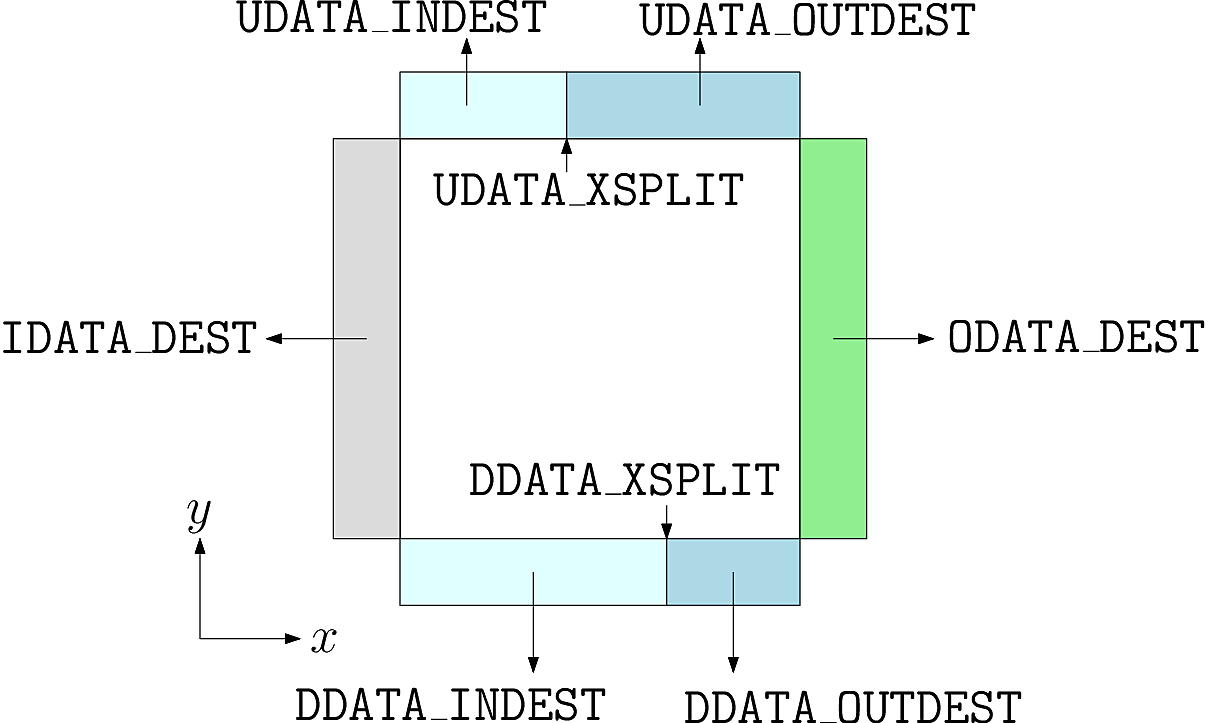
Fig. 7 Communication of guard cells in BOUT++. Boundaries in X have only one neighbour each, but boundaries in Y can be split into two, allowing branch cuts#
In the Y direction, each boundary region (Up and Down in Y)
can be split into two, with 0 <= x < UDATA_XSPLIT going to the
processor index UDATA_INDEST, and UDATA_INDEST <= x < LocalNx going
to UDATA_OUTDEST. Similarly for the Down boundary. Since there are
no branch-cuts in the X direction, there is just one destination for the
Inner and Outer boundaries. In all cases a negative
processor number means that there’s a domain boundary so no
communication is needed.
The communication control variables are set in the
BoutMesh::topology() function, in
src/mesh/impls/bout/boutmesh.cxx. First the function
default_connections sets the topology to be a rectangle.
To change the topology, the function BoutMesh::set_connection() checks
that the requested branch cut is on a processor boundary, and changes
the communications consistently so that communications are two-way and
there are no “dangling” communications.
3D variables#
BOUT++ was originally designed for tokamak simulations where the input equilibrium varies only in X-Y, and Z is used as the axisymmetric toroidal angle direction. In those cases, it is often convenient to have input grids which are only 2D, and allow the Z dimension to be specified independently, such as in the options file. The problem then is how to store 3D variables in the grid file?
Two representations are now supported for 3D variables:
A Fourier representation. If the size of the toroidal domain is not specified in the grid file (
nzis not defined), then 3D fields are stored as Fourier components. In the Z dimension the coefficients must be stored as\[[n = 0, n = 1 (\textrm{real}), n = 1 (\textrm{imag}), n = 2 (\textrm{real}), n = 2 (\textrm{imag}), \ldots ]\]where \(n\) is the toroidal mode number. The size of the array must therefore be odd in the Z dimension, to contain a constant (\(n=0\)) component followed by real/imaginary pairs for the non-axisymmetric components.
If you are using IDL to create a grid file, there is a routine in
tools/idllib/bout3dvar.profor converting between BOUT++’s real and Fourier representation.Real space, as values on grid points. If
nzis set in the grid file, then 3D variables in the grid file must have sizenx\(\times\)ny\(\times\)nz. These are then read in directly intoField3Dvariables as required.
From EFIT files#
A separate tool (in python) called Hypnotoad has been developed to create BOUT++ input files from R-Z equilibria. This can read EFIT ’g’ (geqdsk) files, find flux surfaces, and calculate metric coefficients.
From ELITE and GATO files#
Currently conversions exist for ELITE .eqin and GATO dskgato
equilibrium files. Conversion of these into BOUT++ input grids is in two
stages: In the first, both these input files are converted into a common
NetCDF format which describes the Grad-Shafranov equilibrium. These
intermediate files are then converted to BOUT++ grids using an
interactive IDL script.
Generating equilibria#
The directory tokamak_grids/shifted_circle contains IDL code to
generate shifted circle (large aspect ratio) Grad-Shafranov equilibria.
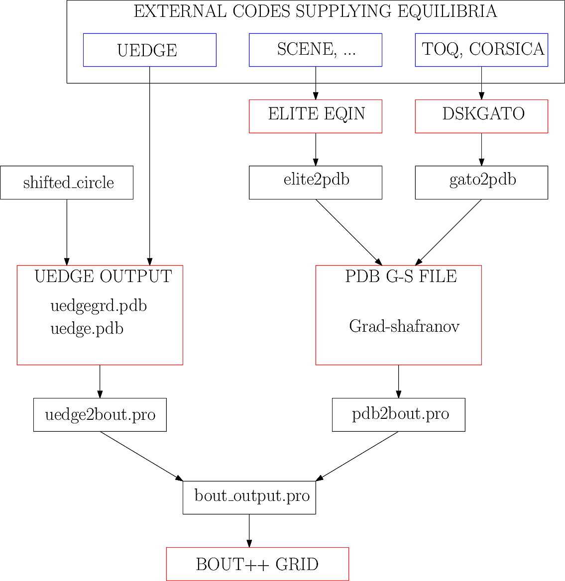
Fig. 8 IDL routines and file formats used in taking output from different codes and converting into input to BOUT++.#
Zoidberg grid generator#
The Zoidberg grid generator creates inputs for the Flux Coordinate Independent (FCI) parallel transform (section Parallel Transforms). The domain is divided into a set of 2D grids in the X-Z coordinates, and the magnetic field is followed along the Y coordinate from each 2D grid to where it either intersects the forward and backward grid, or hits a boundary.
A simple code which creates an output file is:
import zoidberg

# Define the magnetic field
field = zoidberg.field.Slab()
# Define the grid points
grid = zoidberg.grid.rectangular_grid(10,10,10)
# Follow magnetic fields from each point
maps = zoidberg.make_maps(grid, field)
# Write everything to file - with default option for gridfile and metric2d
zoidberg.write_maps(grid, field, maps, gridfile="grid.fci.nc", metric2d=True)
As in the above code, creating an output file consists of the following steps:
Define a magnetic field
Define the grid points. This can be broken down into:
Define 2D “poloidal” grids
Form a 3D grid by putting 2D grids together along the Y direction
Create maps from each 2D grid to its neighbours
Save grids, fields and maps to file
Each of these stages can be customised to handle more complicated
magnetic fields, more complicated grids, and particular output
formats. Details of the functionality available are described in
sections below, and there are several examples in the
examples/zoidberg directory.
Rectangular grids#
An important input to Zoidberg is the size of the domain in Y, and
whether the domain is periodic in Y. By default rectangular_grid makes
a non-periodic rectangular box which is of length 10 in the Y direction.
This means that there are boundaries at \(y=0\) and at \(y=10\).
rectangular_grid puts the y slices at equally spaced intervals, and puts
the first and last points half an interval away from boundaries in y.
In this case with 10 points in y (second argument to rectangular_grid(nx,ny,nz))
the y locations are \(\left(0.5, 1.5, 2.5, \ldots, 9.5\right)\).
At each of these y locations rectangular_grid defines a rectangular 2D poloidal grid in
the X-Z coordinates, by default with a length of 1 in each direction and centred on \(x=0,z=0\).
These 2D poloidal grids are then put together into a 3D Grid. This process can be customised
by separating step 2 (the rectangular_grid call) into stages 2a) and 2b).
For example, to create a periodic rectangular grid we could use the following:
import numpy as np

# Create a 10x10 grid in X-Z with sides of length 1
poloidal_grid = zoidberg.poloidal_grid.RectangularPoloidalGrid(10, 10, 1.0, 1.0)
# Define the length of the domain in y
ylength = 10.0
# Define the y locations
ycoords = np.linspace(0.0, ylength, 10, endpoint=False)
# Create the 3D grid by putting together 2D poloidal grids
grid = zoidberg.grid.Grid(poloidal_grid, ycoords, ylength, yperiodic=True)
In the above code the length of the domain in the y direction needs to be given to Grid
so that it knows where to put boundaries (if not periodic), or where to wrap the domain
(if periodic). The array of y locations ycoords can be arbitrary, but note that finite
difference methods (like FCI) work best if grid point spacing varies smoothly.
A more realistic example is creating a grid for a MAST tokamak equilibrium from a G-Eqdsk
input file (this is in examples/zoidberg/tokamak.py):
import numpy as np
import zoidberg

field = zoidberg.field.GEQDSK("g014220.00200") # Read magnetic field

grid = zoidberg.grid.rectangular_grid(100, 10, 100,
       1.5-0.1, # Range in R (max - min)
       2*np.pi, # Toroidal angle
       3., # Range in Z
       xcentre=(1.5+0.1)/2, # Middle of grid in R
       yperiodic=True) # Periodic in toroidal angle

# Create the forward and backward maps
maps = zoidberg.make_maps(grid, field)

# Save to file
zoidberg.write_maps(grid, field, maps, gridfile="grid.fci.nc")

# Plot grid points and the points they map to in the forward direction
zoidberg.plot.plot_forward_map(grid, maps)
In the last example only one poloidal grid was created (a RectangularPoloidalGrid)
and then re-used for each y slice. We can instead define a different grid for each y
position. For example, to define a grid which expands along y (for some reason) we could do:
ylength = 10.0
ycoords = np.linspace(0.0, ylength, 10, endpoint=False)
# Create a list of poloidal grids, one for each y location
poloidal_grids = [ RectangularPoloidalGrid(10, 10, 1.0 + y/10., 1.0 + y/10.)
                   for y in ycoords ]
# Create the 3D grid by putting together 2D poloidal grids
grid = zoidberg.grid.Grid(poloidal_grids, ycoords, ylength, yperiodic=True)
Note: Currently there is an assumption that the number of X and Z points is the
same on every poloidal grid. The shape of the grid can however be completely
different. The construction of a 3D Grid is the same in all cases, so for now
we will concentrate on producing different poloidal grids.
More general grids#
The FCI technique is not restricted to rectangular grids, and in particular
Zoidberg can handle structured grids in an annulus with quite complicated shapes.
The StructuredPoloidalGrid class handles quite general geometries,
but still assumes that the grid is structured and logically rectangular.
Currently it also assumes that the z index is periodic.
One way to create this grid is to define the grid points manually e.g.:
import numpy as np
import zoidberg

# First argument is minor radius, second is angle
r,theta = np.meshgrid(np.linspace(1,2,10),
                      np.linspace(0,2*np.pi, 10),
                      indexing="ij")

R = r * np.sin(theta)
Z = r * np.cos(theta)

poloidal_grid = zoidberg.poloidal_grid.StructuredPoloidalGrid(R,Z)
For more complicated shapes than circles, Zoidberg comes with an elliptic grid generator which needs to be given only the inner and outer boundaries:
import zoidberg

inner = zoidberg.rzline.shaped_line(R0=3.0, a=0.5,
                         elong=1.0, triang=0.0, indent=1.0,
                         n=50)

outer = zoidberg.rzline.shaped_line(R0=2.8, a=1.5,
                         elong=1.0, triang=0.0, indent=0.2,
                         n=50)

poloidal_grid = zoidberg.poloidal_grid.grid_elliptic(inner, outer,
                                              100, 100, show=True)
which should produce the figure below:
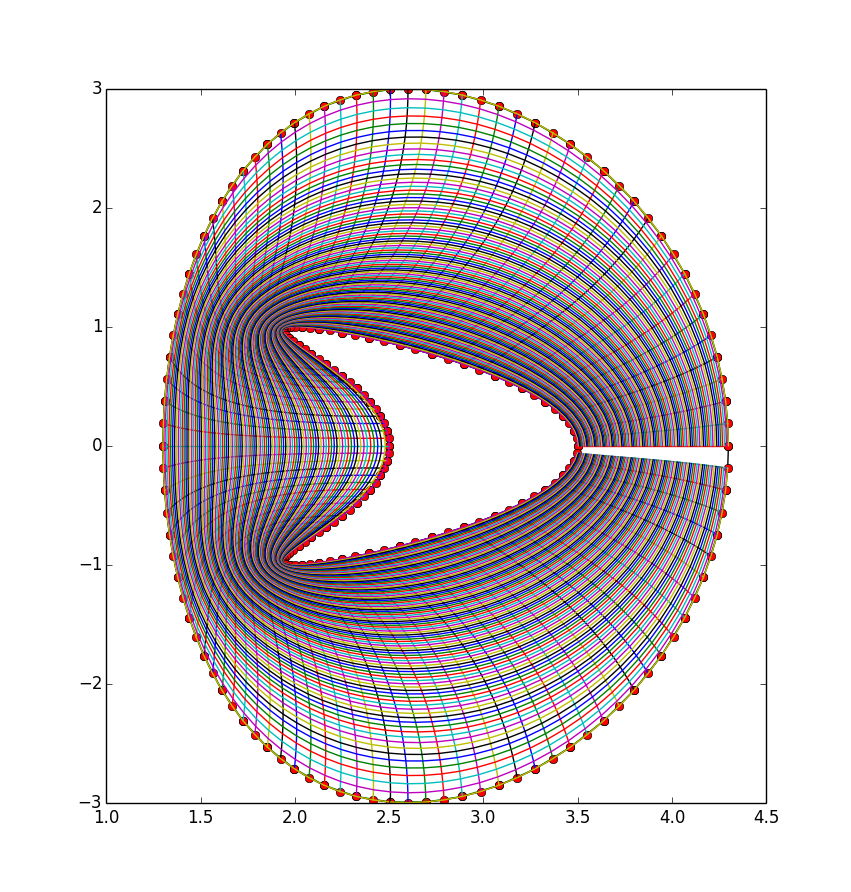
Fig. 9 A grid produced by grid_elliptic from shaped inner and outer lines#
Grids aligned to flux surfaces#
The elliptic grid generator can be used to generate grids
whose inner and/or outer boundaries align with magnetic flux surfaces.
All it needs is two RZline objects as generated by zoidberg.rzline.shaped_line,
one for the inner boundary and one for the outer boundary.
RZline objects represent periodic lines in R-Z (X-Z coordinates), with
interpolation using splines.
To create an RZline object for a flux surface we first need to find
where the flux surface is. To do this we can use a Poincare plot: Start at a point
and follow the magnetic field a number of times around the periodic y direction
(e.g. toroidal angle). Every time the field line reaches a y location of interest,
mark the position to build up a scattered set of points which all lie on the same
flux surface.
At the moment this will not work correctly for slab geometries, but expects closed flux surfaces such as in a stellarator or tokamak. A simple test case is a straight stellarator:
import zoidberg
field = zoidberg.field.StraightStellarator(I_coil=0.4, yperiod=10)
By default StraightStellarator calculates the magnetic field due to four coils which spiral around
the axis at a distance \(r=0.8\) in a classical stellarator configuration. The yperiod
argument is the period in y after which the coils return to their starting locations.
To visualise the Poincare plot for this stellarator field, pass the MagneticField object
to zoidberg.plot.plot_poincare, together with start location(s) and periodicity information:
zoidberg.plot.plot_poincare(field, 0.4, 0.0, 10.0)
which should produce the following figure:
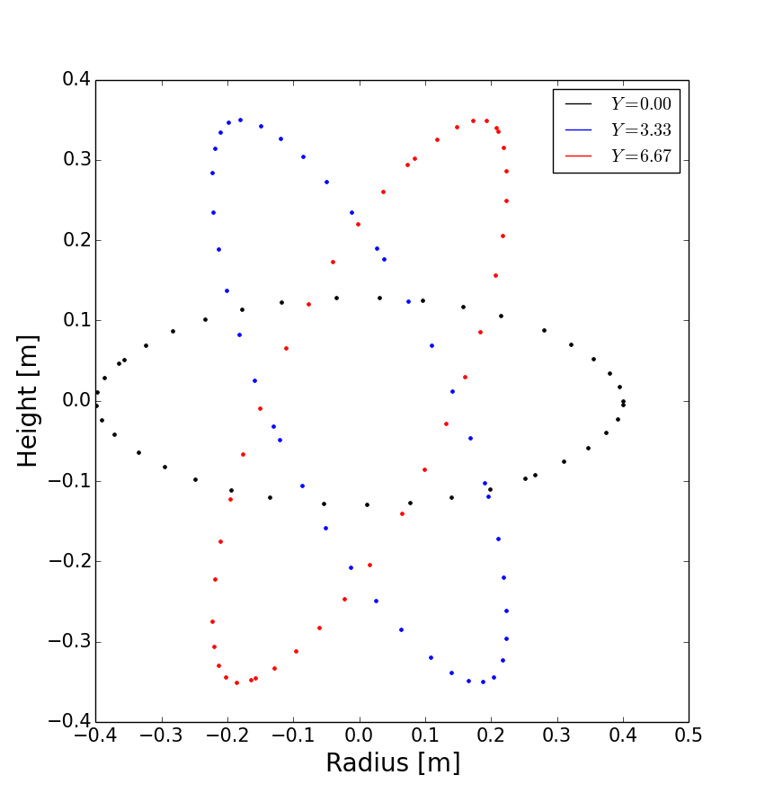
Fig. 10 Poincare map of straight stellarator showing a single flux surface. Each colour corresponds to a different x-z plane in the y direction.#
The inputs here are the starting location \(\left(x,z\right) = \left(0.4, 0.0\right)\),
and the periodicity in the y direction (10.0). By default this will
integrate from this given starting location 40 times (revs option) around the y domain (0 to 10).
To create an RZline from these Poincare plots we need a
list of points in order around the line. Since the points
on a flux surface in a Poincare will not generally be in order
we need to find the best fit i.e. the shortest path which passes through all the points without crossing itself. In general
this is a known hard problem
but fortunately in this case the nearest neighbour algorithm seems to be quite robust provided there are enough points.
An example of calculating a Poincare plot on a single y slice (y=0) and producing an RZline is:
from zoidberg.fieldtracer import trace_poincare
rzcoord, ycoords = trace_poincare(field, 0.4, 0.0, 10.0,
                                  y_slices=[0])

R = rzcoord[:,0,0]
Z = rzcoord[:,0,1]

line = zoidberg.rzline.line_from_points(R, Z)

line.plot()
Note: Currently there is no checking that the line created is a good solution. The line
could cross itself, but this has to be diagnosed manually at the moment. If the line is not a good
approximation to the flux surface, increase the number of points by setting the revs keyword
(y revolutions) in the trace_poincare call.
In general the points along this line are not evenly
distributed, but tend to cluster together in some regions and have large gaps in others.
The elliptic grid generator places grid points on the boundaries
which are uniform in the index of the RZline it is given.
Passing a very uneven set of points will therefore result in
a poor quality mesh. To avoid this, define a new RZline
by placing points at equal distances along the line:
line = line.equallySpaced()
The example zoidberg/straight-stellarator-curvilinear.py puts the above methods together to create a grid file for a straight stellarator.
Sections below now describe each part of Zoidberg in more detail. Further documentation of the API can be found in the docstrings and unit tests.
Magnetic fields#
The magnetic field is represented by a MagneticField class, in zoidberg.field.
Magnetic fields can be defined in either cylindrical or Cartesian coordinates:
In Cartesian coordinates all (x,y,z) directions have the same units of length
In cylindrical coordinates the y coordinate is assumed to be an angle, so that the distance in y is given by \(ds = R dy\) where \(R\) is the major radius.
Which coordinate is used is controlled by the Rfunc method, which should return the
major radius if using a cylindrical coordinate system.
Should return None for a Cartesian coordinate system (the default).
Several implementations inherit from MagneticField, and provide:
Bxfunc, Byfunc, Bzfunc which give the components of the magnetic field in
the x,y and z directions respectively. These should be in the same units (e.g. Tesla) for
both Cartesian and cylindrical coordinates, but the way they are integrated changes depending
on the coordinate system.
Using these functions the MagneticField class provides a Bmag method and field_direction
method, which are called by the field line tracer routines (in zoidberg.field_tracer).
Slabs and curved slabs#
The simplest magnetic field is a straight slab geometry:
import zoidberg
field = zoidberg.field.Slab()
By default this has a magnetic field \(\mathbf{B} = \left(0, 1, 0.1 + x\right)\).
A variant is a curved slab, which is defined in cylindrical coordinates and has a given major radius (default 1):
import zoidberg
field = zoidberg.field.CurvedSlab()
Note that this uses a large aspect-ratio approximation, so the major radius is constant across the domain (independent of x).
Straight stellarator#
This is generated by four coils with alternating currents arranged on the edge of a circle, which spiral around the axis:
import zoidberg
field = zoidberg.field.StraightStellarator()
Note
This requires Sympy to generate the magnetic field, so if unavailable an exception will be raised
G-Eqdsk files#
This format is commonly used for axisymmetric tokamak equilibria, for example output from EFIT equilibrium reconstruction. It consists of the poloidal flux psi, describing the magnetic field in R and Z, with the toroidal magnetic field Bt given by a 1D function f(psi) = R*Bt which depends only on psi:
import zoidberg
field = zoidberg.field.GEQDSK("gfile.eqdsk")
VMEC files#
The VMEC format describes 3D magnetic fields in toroidal geometry, but only includes closed flux surfaces:
import zoidberg
field = zoidberg.field.VMEC("w7x.wout")
Plotting the magnetic field#
Routines to plot the magnetic field are in zoidberg.plot. They include Poincare plots
and 3D field line plots.
For example, to make a Poincare plot from a MAST equilibrium:
import numpy as np
import zoidberg
field = zoidberg.field.GEQDSK("g014220.00200")
zoidberg.plot.plot_poincare(field, 1.4, 0.0, 2*np.pi, interactive=True)
This creates a flux surface starting at \(R=1.4\) and \(Z=0.0\). The fourth input (2*np.pi) is
the periodicity in the \(y\) direction. Since this magnetic field is symmetric in y (toroidal angle),
this parameter only affects the toroidal planes where the points are plotted.
The interactive=True argument to plot_poincare generates a new set of points for every click
on the plot window.
Creating poloidal grids#
The FCI technique is used for derivatives along the magnetic field (in Y), and doesn’t restrict the form of the grid in the X-Z poloidal planes. A 3D grid created by Zoidberg is a collection of 2D planes (poloidal grids), connected together by interpolations along the magnetic field.To define a 3D grid we first need to define the 2D poloidal grids.
Two types of poloidal grids can currently be created: Rectangular grids, and curvilinear structured grids. All poloidal grids have the following methods:
getCoordinate()which returns the real space (R,Z) coordinates of a given (x,z) index, or derivatives thereoffindIndex()which returns the (x,z) index of a given (R,Z) coordinate which in general is floating pointmetric()which returns the 2D metric tensorplot()which plots the grid
Rectangular grids#
To create a rectangular grid, pass the number of points and lengths in the x and z directions
to RectangularPoloidalGrid:
import zoidberg

rect = zoidberg.poloidal_grid.RectangularPoloidalGrid( nx, nz, Lx, Lz )
By default the middle of the rectangle is at \(\left(R,Z\right) = \left(0,0\right)\)
but this can be changed with the Rcentre and Zcentre options.
Curvilinear structured grids#
To create the structured curvilinear grids inner and outer lines are needed
(two RZline objects). The shaped_line function creates RZline shapes
with the following formula:
where \(R_0\) is the major radius, \(a\) is the minor radius,
\(\epsilon\) is the elongation (elong), \(\delta\) the triangularity (triang), and \(b\) the indentation (indent).