PETSc interface
The Portable, Extensible Toolkit for Scientific Computation (PETSc) provides a large collection of
numerical routines and solvers. It is used in BOUT++ for
Time integration and Laplacian inversion. However, it provides
quite a low-level C interface which is often difficult to use and
bears little resemblance to the data model of BOUT++. This is
particularly the case when making use of the Mat and Vec data-types
for linear solvers (such as the Laplacian inversions). Doing so
requires the developer to:
Flatten a
Fieldinto a 1-D PETScVecobject.Must decide which guard cells to include in
VecMust convert between BOUT++ indices (local) and indices used in PETSc
Vec(global)
Use a PETSc
Matobject to represent a finite-difference operator.Again, must convert between local and global indices
Must determine sparsity pattern of matrix
If taking field-aligned derivatives, must perform interpolation
Call a Krylov solver with a preconditioner.
Convert the resulting
Vecobject back into aField.
These tasks are error-prone and have historically been re-implemented each time a PETSc solver is to be used. An interface to PETSc has now been added which greatly simplifies its use. Furthermore, it has been thoroughly unit-tested which should ensure improved reliability.
Overall Structure
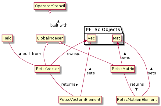
Fig. 23 A UML diagram showing the design of the PETSc interface and the relationships between different components.
Based on the finite difference operator being inverted, a user
constructs an OperatorStencil object which is used to describe the
interdependencies between cells in the grid. This is used when
constructing a GlobalIndexer to work out which cells should be
included in a Vec object. If needed, it will also be used to work
out the sparsity pattern of a matrix. PetscVector and PetscMatrix
objects are constructed from a GlobalIndexer and wrap the PETSc
Vec and Mat objects, respectively. They provide routines for
accessing individual elements of the vector/matrix using
PetscVector::Element and PetscMatrix::Element objects. All of
these classes are templates. OperatorStencil works for SpecificInd
types (Ind3D, Ind2D, IndPerp), while the remaining classes
work for the various Field types.
OperatorStencil
This data type describes the strucutre of the finite difference
operator which is to be inverted. It uses a number of small
helper-types to do this (see Fig. 24), the most
important of which is the IndexOffset. This is a simple structure
which represents an offset from a SpecificInd<> type. It can be
added to or subtracted from SpecificInd<> objects, returning
an index which is suitably offset.
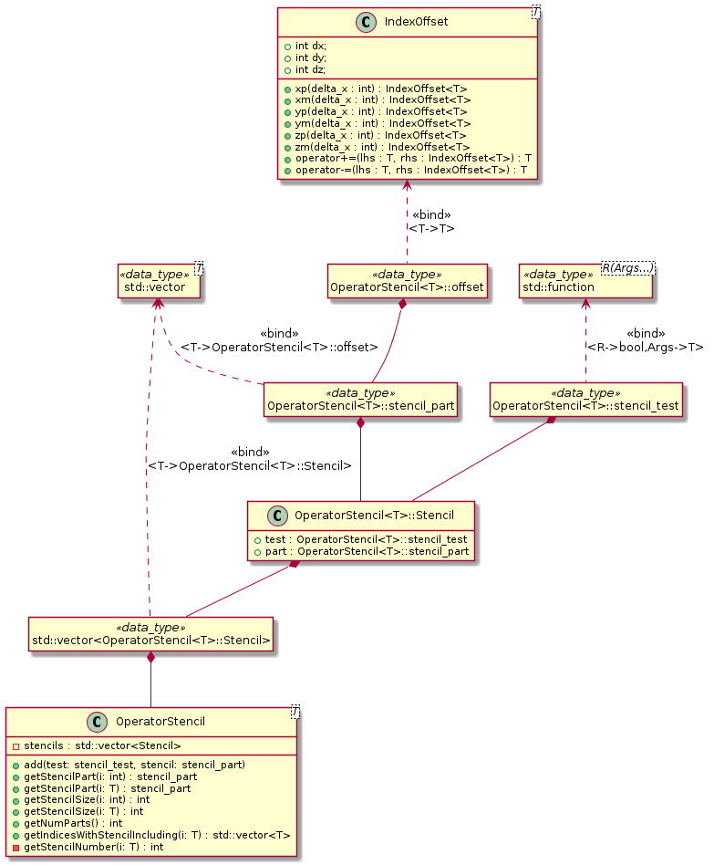
Fig. 24 UML diagram describing the structure of the OperatorStencil class.
Vectors of IndexOffset objects are coupled with tests which take a
SpecificInd<> as an argument and return a boolean result
indicating whether the offsets describe the finite difference stencil
at that location. The OperatorStencil class contains a vector of
these pairs. When the stencil is requested for a given index, the
vector gets traversed in order, with offsets returned from the first
passing test. Pairs of tests and offsets are placed in the
OperatorStencil object using the add() method. It will
generally not be necessary for you to use any of the other methods on
this class unless you are doing further development work on the PETSc
interface.
Consider a 2-D Laplacian operator with the discretisation
\(\nabla^2 f(i,j) = \frac{f(i+1,j) - 2f(i,j) + f(i-1,j)}{\Delta x^2} + \frac{f(i,j+1) - 2f(i,j) + f(i,j-1)}{\Delta y^2}\)
and Neumann boundary conditions. Then an appropriate stencil could be created using the following code.
OperatorStencil<Ind2D> stencil;
OffsetInd2D zero;

// Add Laplace stencil for interior grid points
stencil.add([xs = localmesh->xstart, xe = localmesh->xend, ys = localmesh->ystart,
             ye = localmesh->yend](Ind2D ind) -> bool {
               return ind.x() >= xs && ind.x() <= xe &&
                      ind.y() >= ys && ind.y() <= ye;},
            {zero, zero.xp(), zero.xm(), zero.yp(), zero.ym()});

// Add first-order differences for Neumann boundaries
// Inner X
stencil.add([xs = localmesh->xstart](Ind2D ind) -> bool {
               return ind.x() < xs; }, {zero, zero.xp()});
// Outer X
stencil.add([xe = localmesh->xend](Ind2D ind) -> bool {
               return ind.x() > xe; }, {zero, zero.xm()});
// Lower Y
stencil.add([ys = localmesh->ystart](Ind2D ind) -> bool {
               return ind.y() < ys; }, {zero, zero.yp()});
// Upper Y
stencil.add([ye = localmesh->yend](Ind2D ind) -> bool {
               return ind.y() > ye; }, {zero, zero.ym()});
GlobalIndexer
Using an OperatorStencil, the GlobalIndexer constructor can
determine which cells should be included in the PETSc Vec object
representing a Field. All interior cells are always
included. Boundary cells which are required by the stencil to compute
the operation on internal cells are also included. A globally-unique
index is assigned to each cell which is meant to be included and the
communication routines on the Mesh type are used to determine the
indices in guard cells. There must be a unique GlobalIndexer object
for each Mesh and OperatorStencil pair. You will need to pass a
std::shared_ptr<GlobalIndexer> object (with type-alias
IndexerPtr) when constructing PetscVector and PetscMatrix
objects. As the process of creating a GlobalIndexer is quite
expensive and each one contains a field of indices, you will not want
to create any copies (hence the use of std::shared_ptr).
In comparison to initialising an OperatorStencil object, creating
a GlobalIndexer is quite simple. The constructor takes 3 arguments,
two of which are optional:
A pointer to the
Meshobject for the indexerAn
OperatorStencil; if absent then the indexer will not include any guard cells in the PETSc objects and will not compute matrix sparsity patternsA boolean specifying whether communication of indices in guard cells will be performed in the constructor; defaults to
true, otherwise will need to call theinitialise()method prior to use (you would generally only do that if creating a fake indexer for testing purposes)
Continuing on from the previous example, the code below shows how to
create a GlobalIndexer.
IndexerPtr<Field2D> indexer =
    std::make_shared<GlobalIndexer<Field2D>>(localmesh, stencil);
The GlobalIndexer class provides Region<> objects which can be
used for iterating over the cells which are included in PETSc Vec
objects (see Iterating over fields). This is useful for setting vector
and matrix elements. The relevant methods are:
getRegionAll()returns a region containing all cells included in the PETSc objectsgetRegionNobndry()contains only the non-guard cells include in the PETSc objects (identical toRGN_NOBNDRY)getRegionBndry()contains only guard cells which are also boundary cellsgetRegionLowerY()contains only guard cells in the lower Y-boundarygetRegionUpperY()contains only guard cells in the upper Y-boundarygetRegionInnerX()contains only guard cells in the inner X-boundarygetRegionOuterX()contains only guard cells in the outer X-boundary
Note that not all guard-cells will be boundary cells; most will just be used for communication between processors.
PetscVector
This class wraps PETSc Vec objects, split across multiple
processors. The constructors/destructors ensure memory will be
allocated/freed as necessary. To create a new vector, pass a Field
and IndexerPtr to the constructor. This will create a Vec
object which is split between processors. The IndexerPtr will be
used to convert between the local BOUT++ coordinate system and the
global PETSc indices used to access elements of the Vec
object. The values in the Field will be copied into the
Vec. The user can set individual elements using local BOUT++
indices and the parentheses operator (). Once this is done, call
the assemble() method. Elements can be set using either assignment
(=) or in-place addition (+=). However, as in PETSc itself,
these operations can not be mixed, unless there is call to
assemble() in between. A PetscVector can be converted back to a
Field object using the toField() method.
Below is an example of creating a vector which could be used as input for a linear solver.
Field2D rhs_vals; // Assume this is initialised with some data
PetscVector<Field2D> rhs_vec(rhs_vals, indexer);

// Set boundary values to 0
BOUT_FOR(i, indexer.getRegionBndry()) {
  rhs_vec(i) = 0.;
}
rhs_vec.assemble();
If you plan to do any development of the PETSc interface (or simply wish to understand how it works), see the UML sequence diagram in Fig. 25 for a description of how vector elements are set.
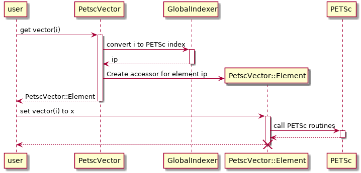
Fig. 25 A UML sequence diagram showing what happens when setting an element
of a PetscVector. The GlobalIndexer is used to convert from the
BOUT++ index to the one used by PETSc. A placeholder
PetscVector::Element object is returned containing the index
and a pointer to the Vec object. The assignment operator on
this class makes a call to the PETSc routine VecSetValue.
PetscMatrix
This class wraps a PETSc Mat object, including managing memory in
its constructors and destructor. This is a sparse matrix using the AIJ
storage method. It is split across multiple processors. The
PetscMatrix object is constructed from a IndexerPtr object;
unlike for a PetscVector it would not make sense to copy data from a
Field into a PetscMatrix object in the constructor. If the
GlobalIndexer has this data available, the sparsity pattern of the
Mat object will be passed to PETSc. This allows memory to be
pre-allocated for it by PETSc, which dramatically improved
performance.
As with PetscVector objects, individual elements of a PetscMatrix
can be accessed using BOUT++ indices and the parentheses operator,
except that now two indices are required (corresponding to the row and
column of the matrix). These elements can be set using either
assignment or in-place addition. Once again, these two modes can not
be mixed unless the matrix is assembled in between, this time using
the partialAssemble() method. Before using the matrix a call must
be made to the assemble() method. This can be used between modes
of setting matrix elements as well, but is slower than
partialAssemble().
It is possible to use one of these matrix objects to represent
finite-difference operations in the field-aligned direction. Much like
when working with Fields (see Parallel Transforms), this
can be achieved using the yup() and ydown() methods. These
return a shallow-copy of the matrix object, with a flag indicating it
is offset up or downwards in the y-direction. When using the
parentheses operator to get a particular matrix element, the mesh’s
ParallelTransform object will be queried to find the positions and
weights needed to interpolate values onto field lines. This
information is stored in the PetscMatrix::Element object which is
returned. When that object is assigned to, it will set multiple matrix
elements in the specified row, corresponding to each cell used to
interpolate the along-field value. Note that the same cell might be
used for interpolating more than one along-field value and it is thus
possible you would end up overwriting a matrix element that you
need. As such, you should always use in-place addition when using
yup() and ydown().
Putting all of this together, a matrix can be created corresponding to the Laplace operator defined in OperatorStencil.
PetscMatrix<Field2D> matrix(indexer);
Field2D &dx = localmesh->getCoordinates()->dx,
        &dy = localmesh->getCoordinates()->dy;

// Set up x-derivatives
BOUT_FOR(i, indexer->getRegionNobndry()) {
  matrix(i, i.xp()) = 1./SQ(dx[i]);
  matrix(i, i) = -2./SQ(dx[i]);
  matrix(i, i.xm()) = 1./SQ(dx[i]);
}
BOUT_FOR(i, indexer->getRegionInnerX()) {
  matrix(i, i.xp()) =  1./dx[i];
  matrix(i, i) = -1./dx[i];
}
BOUT_FOR(i, indexer->getRegionOuterX()) {
  matrix(i, i) =  1./dx[i];
  matrix(i, i.xm()) = -1./dx[i];
}
matrix.partialAssemble();

// Set up y-derivatives
BOUT_FOR(i, indexer->getRegionNobndry()) {
  matrix.yup()(i, i.yp()) += 1./SQ(dy[i]);
  matrix(i, i) += -2./SQ(dy[i]);
  matrix.ydown()(i, i.ym()) += 1/SQ(dy[i]);
}
BOUT_FOR(i, indexer->getRegionLowerY()) {
  matrix.yup()(i, i.yp()) += 1./dy[i];
  matrix(i, i) += -1./dy[i];
}
BOUT_FOR(i, indexer->getRegionUpperY()) {
  matrix(i, i) += 1./dy[i];
  matrix.ydown()(i, i.ym()) += -1./dy[i];
}
matrix.assemble();
Use With Other Parts of PETSc
At present, only the Mat and Vec objects in PETSc have been
wrapped. This is because they are by far the most difficult components
to use and benefit the most from providing this interface. While in
future a C++ interface may be provided to other components of PETSc,
for the time being it is not too difficult to use the raw C API. This
can be done by getting a pointer to the raw Mat and Vec
objects using the PetscMatrix::get() and PetscVector::get()
methods. For example, to set up and use a linear solver for the
problem in previous sections could be done as below:
MatSetBlockSize(*matrix.get(), 1);
KSP solver;
KSPSetOperators(solver, *matrix.get(), *matrix.get());
KSPSetType(solver, "richardson")
KSPRichardsonSetScale(solver, 1.0)
KSPSetTolerances(solver, 1e-8, 1e-8, 1e6, 100000);
KSPSetInitialGuessNonzero(solver, PETSC_TRUE);

// Set up an algebraic multigrid preconditioner
PC precond;
KSPGetPC(solver, &precond);
PCSetType(precond, PCGAMGAGG);
PCGAMGSetSymGraph(precond, PETSC_TRUE);

PetscVector<Field2D> guess = rhs_vec;
guess.assemble();

KSPSolve(solver, *rhs_vec.get(), *guess.get());
KSPConvergedReason reason;
KSPGetConvergedReason(solver, &reason);
if (reason <= 0) {
  throw BoutException("PETSc solver failed"):
}

Field2D solution = guess.toField();