Differential operators

There are a huge number of possible ways to perform differencing in computational fluid dynamics, and BOUT++ is intended to be able to implement a large number of them. This means that the way differentials are handled internally is quite involved; see the developer’s manual for full gory details. Much of the time this detail is not all that important, and certainly not while learning to use BOUT++. Default options are therefore set which work most of the time, so you can start using the code without getting bogged down in these details.

In order to handle many different differencing methods and operations, many layers are used, each of which handles just part of the problem. The main division is between differencing methods (such as 4th-order central differencing), and differential operators (such as \(\nabla_{||}\)).

Differencing methods

Methods are typically implemented on 5-point stencils (although exceptions are possible) and are divided into three categories:

• Central-differencing methods, for diffusion operators \(\frac{df}{dx}\), \(\frac{d^2f}{dx^2}\). Each method has a short code, and currently include

  • C2: 2\(^{nd}\) order \(f_{-1} - 2f_0 + f_1\)

  • C4: 4\(^{th}\) order \((-f_{-2} + 16f_{-1} - 30f_0 + 16f_1 - f_2)/12\)

  • S2: 2\(^{nd}\) order smoothing derivative

  • W2: 2\(^{nd}\) order CWENO

  • W3: 3\(^{rd}\) order CWENO

• Upwinding methods for advection operators \(v_x\frac{df}{dx}\)

  • U1: 1\(^{st}\) order upwinding

  • U2: 2\(^{nd}\) order upwinding

  • U3: 3\(^{rd}\) order upwinding

  • U4: 4\(^{th}\) order upwinding

  • C2: 2\(^{nd}\) order central

  • C4: 4\(^{th}\) order central

  • W3: 3\(^{rd}\) order Weighted Essentially Non-Oscillatory (WENO)

• Flux conserving and limiting methods for terms of the form \(\frac{d}{dx}(v_x f)\)

  • U1: 1\(^{st}\) order upwinding

  • C2: 2\(^{nd}\) order central

  • C4: 4\(^{th}\) order central

Special methods :

• FFT: Classed as a central method, Fourier Transform method in Z

  (axisymmetric) direction only. Currently available for first and second order central difference

• SPLIT: A flux method that splits into upwind and central terms

  \(\frac{d}{dx}(v_x f) = v_x\frac{df}{dx} + f\frac{dv_x}{dx}\)

WENO methods avoid overshoots (Gibbs phenomena) at sharp gradients such as shocks, but the simple 1st-order method has very large artificial diffusion. WENO schemes are a development of the ENO reconstruction schemes which combine good handling of sharp-gradient regions with high accuracy in smooth regions.

The stencil based methods are based by a kernel that combines the data in a stencil to produce a single BoutReal (note upwind/flux methods take extra information about the flow, either a BoutReal or another stencil). It is not anticipated that the user would wish to apply one of these kernels directly so documentation is not provided here for how to do so. If this is of interest please look at include/bout/index_derivs.hxx. Internally, these kernel routines are combined within a functor struct that uses a BOUT_FOR loop over the domain to provide a routine that will apply the kernel to every point, calculating the derivative everywhere. These routines are registered in the appropriate DerivativeStore and identified by the direction of differential, the staggering, the type (central/upwind/flux) and a key such as “C2”. The typical user does not need to interact with this store, instead one can add the following to the top of your physics module:

#include <derivs.hxx>

to provide access to the following routines. These take care of selecting the appropriate method from the store and ensuring the input/output field locations are compatible.

Table 17 Coordinate derivatives

Function	Formula
DDX(f)	\(\partial f / \partial x\)
DDY(f)	\(\partial f / \partial y\)
DDZ(f)	\(\partial f / \partial z\)
D2DX2(f)	\(\partial^2 f / \partial x^2\)
D2DY2(f)	\(\partial^2 f / \partial y^2\)
D2DZ2(f)	\(\partial^2 f / \partial z^2\)
D4DX4(f)	\(\partial^4 f / \partial x^4\)
D4DY4(f)	\(\partial^4 f / \partial y^4\)
D4DZ4(f)	\(\partial^4 f / \partial z^4\)
D2DXDZ(f)	\(\partial^2 f / \partial x\partial z\)
D2DYDZ(f)	\(\partial^2 f / \partial y\partial z\)
VDDX(f, g)	\(f \partial g / \partial x\)
VDDY(f, g)	\(f \partial g / \partial y\)
VDDZ(f, g)	\(f \partial g / \partial z\)
FDDX(f, g)	\(\partial/\partial x( f * g )\)
FDDY(f, g)	\(\partial/\partial x( f * g )\)
FDDZ(f, g)	\(\partial/\partial x( f * g )\)

By default the method used will be the one specified in the options input file (see Differencing methods), but most of these methods can take an optional std::string argument (or a DIFF_METHOD argument - to be deprecated), specifying exactly which method to use.

User registered methods

Note

The following may be considered advanced usage.

It is possible for the user to define their own differencing routines, either by supplying a stencil using kernel or writing their own functor that calculates the differential everywhere. It is then possible to register these methods with the derivative store (for any direction, staggering etc.). For examples please look at include/bout/index_derivs.hxx to see how these approaches work.

Here is a verbose example showing how the C2 method is implemented.

DEFINE_STANDARD_DERIV(DDX_C2, "C2", 1, DERIV::Stanard) {
    return 0.5*(f.p - f.m);
};

Here DEFINE_STANARD_DERIV is a macro that acts on the kernel return 0.5*(f.p - f.m); and produces the functor that will apply the differencing method over an entire field. The macro takes several arguments;

• the first (DDX_C2) is the name of the generated functor – this needs to be unique and allows advanced users to refer to a specific derivative functor without having to go through the derivative store if desired.

• the second ("C2") is the string key that is used to refer to this specific method when registering/retrieving the method from the derivative store.

• the third (1) is the number of guard cells required to be able to use this method (i.e. here the stencil will consist of three values – the field at the current point and one point either side). This can be 1 or 2.

• the fourth (DERIV::Standard) identifies the type of method - here a central method.

Alongside DEFINE_STANDARD_DERIV there’s also DEFINE_UPWIND_DERIV, DEFINE_FLUX_DERIV and the staggered versions DEFINE_STANDARD_DERIV_STAGGERED, DEFINE_UPWIND_DERIV_STAGGERED and DEFINE_FLUX_DERIV_STAGGERED.

To register this method with the derivative store in X and Z with no staggering for both field types we can then use the following code:

produceCombinations<Set<WRAP_ENUM(DIRECTION, X), WRAP_ENUM(DIRECTION, Z)>,
                 Set<WRAP_ENUM(STAGGER, None)>,
                 Set<TypeContainer<Field2D, Field3D>>,
                 Set<DDX_C2>>
 someUniqueNameForDerivativeRegistration(registerMethod{});

For the common case where the user wishes to register the method in X, Y and Z and for both field types we provide the helper macros, REGISTER_DERIVATIVE and REGISTER_STAGGERED_DERIVATIVE which could be used as REGISTER_DERIVATIVE(DDX_C2).

To simplify matters further we provide REGISTER_STANDARD_DERIVATIVE, REGISTER_UPWIND_DERIVATIVE, REGISTER_FLUX_DERIVATIVE, REGISTER_STANDARD_STAGGERED_DERIVATIVE, REGISTER_UPWIND_STAGGERED_DERIVATIVE and REGISTER_FLUX_STAGGERED_DERIVATIVE macros that can define and register a stencil using kernel in a single step. For example:

REGISTER_STANDARD_DERIVATIVE(DDX_C2, "C2", 1, DERIV::Standard) { return 0.5*(f.p-f.m);};

Will define the DDX_C2 functor and register it with the derivative store using key "C2" for all three directions and both fields with no staggering.

Mixed second-derivative operators

Coordinate derivatives commute, as long as the coordinates are globally well-defined, i.e.

\[\begin{split}\frac{\partial}{\partial x} \left(\frac{\partial}{\partial y} f \right) = \frac{\partial}{\partial y} \left(\frac{\partial}{\partial x} f \right) \\ \frac{\partial}{\partial y} \left(\frac{\partial}{\partial z} f \right) = \frac{\partial}{\partial z} \left(\frac{\partial}{\partial y} f \right) \\ \frac{\partial}{\partial z} \left(\frac{\partial}{\partial x} f \right) = \frac{\partial}{\partial x} \left(\frac{\partial}{\partial z} f \right)\end{split}\]

When using paralleltransform = shifted or paralleltransform = fci (see Parallel Transforms) we do not have globally well-defined coordinates. In those cases the coordinate systems are field-aligned, but the grid points are at constant toroidal angle. The field-aligned coordinates are defined locally, on planes of constant \(y\). There are different coordinate systems for each plane. However, within each local coordinate system the derivatives do commute. \(y\)-derivatives are taken in the local field-aligned coordinate system, so mixed derivatives are calculated as

D2DXDY(f) = DDX(DDY(f))
D2DYDZ(f) = DDZ(DDY(f))

This order is simpler – the alternative is possible. Using second-order central difference operators for the y-derivatives we could calculate (not worring about communications or boundary conditions here)

Field3D D2DXDY(Field3D f) {
  auto result{emptyFrom(f)};
  auto& coords = *f.getCoordinates()

  auto dfdx_yup = DDX(f.yup());
  auto dfdx_ydown = DDX(f.ydown());

  BOUT_FOR(i, f.getRegion()) {
    result[i] = (dfdx_yup[i.yp()] - dfdx_ydown[i.ym()]) / (2. * coords.dy[i])
  }

  return result;
}

This would give equivalent results to the previous form [1] as yup and ydown give the values of f one grid point along the magnetic field in the local field-aligned coordinate system.

The \(x\mathrm{-}z\) derivative is unaffected as it is taken entirely on a plane of constant \(y\) anyway. It is evaluated as

D2DXDZ(f) = DDZ(DDX(f))

As the z-direction is periodic and the z-grid is not split across processors, DDZ does not require any guard cells. By taking DDZ second, we do not have to communicate or set boundary conditions on the result of DDX or DDY before taking DDZ.

The derivatives in D2DXDY(f) are applied in two steps. First dfdy = DDY(f) is calculated; dfdy is communicated and has a boundary condition applied so that all the x-guard cells are filled. The boundary condition is free_o3 by default (3rd order extrapolation into the boundary cells), but can be specified with the fifth argument to D2DXDY (see Boundary conditions for possible options). Second DDX(dfdy) is calculated, and returned from the function.

[1]

Equivalent but not exactly the same numerically. Expanding out the derivatives in second-order central-difference form shows that the two differ in the grid points at which they evaluate dx and dy. As long as the grid spacings are smooth this should not affect the order of accuracy of the scheme (?).

Non-uniform meshes

examples/test-nonuniform seems to not work? Setting non_uniform = true in the BOUT.inp options file enables corrections to second derivatives in \(X\) and \(Y\). This correction is given by writing derivatives as:

\[{{\frac{\partial f}{\partial x}}} \simeq \frac{1}{\Delta x} {{\frac{\partial f}{\partial i}}}\]

where \(i\) is the cell index number. The second derivative is therefore given by

\[\frac{\partial^2 f}{\partial x^2} \simeq \frac{1}{\Delta x^2}\frac{\partial^2 f}{\partial i^2} + \frac{1}{\Delta x}{{\frac{\partial f}{\partial x}}} \cdot {{\frac{\partial }{\partial i}}}(\frac{1}{\Delta x})\]

The correction factor \(\partial/\partial i(1/\Delta x)\) can be calculated automatically, but you can also specify d2x in the grid file which is

\[\texttt{d2x} = {{\frac{\partial \Delta x}{\partial i}}} = \frac{\partial^2 x}{\partial i^2}\]

The correction factor is then calculated from d2x using

\[{{\frac{\partial }{\partial i}}}(\frac{1}{\Delta x}) = -\frac{1}{\Delta x^2} {{\frac{\partial \Delta x}{\partial i}}}\]

Note: There is a separate switch in the Laplacian inversion code, which enables or disables non-uniform mesh corrections.

General operators

These are differential operators which are for a general coordinate system.

\[\begin{split}\begin{array}{rclrcl} \mathbf{v} =& \nabla f &\qquad {\texttt{Vector}} =& {\texttt{Grad(Field)}} \\ f =& \nabla\cdot\mathbf{a} &\qquad {\texttt{Field}} =& {\texttt{Div(Vector)}} \\ \mathbf{v} =& \nabla\times\mathbf{a} &\qquad {\texttt{Vector}} =& {\texttt{Curl(Vector)}} \\ f =& \mathbf{v}\cdot\nabla g &\qquad {\texttt{Field}} =& {\texttt{V\_dot\_Grad(Vector, Field)}} \\ \mathbf{v} =& \mathbf{a}\cdot\nabla\mathbf{c} &\qquad {\texttt{Vector}} =& {\texttt{V\_dot\_Grad(Vector, Vector)}} \\ f =& \nabla^2 f &\qquad {\texttt{Field}} =& {\texttt{Laplace(Field)}} \end{array}\end{split}\]

\[\begin{split}\nabla\phi =& {{\frac{\partial \phi}{\partial u^i}}}\nabla u^i \rightarrow (\nabla\phi)_i = {{\frac{\partial \phi}{\partial u^i}}} \\ \nabla\cdot A =& = \frac{1}{J}{{\frac{\partial }{\partial u^i}}}(Jg^{ij}A_j) \\ \nabla^2\phi =& G^j{{\frac{\partial \phi}{\partial u^i}}} + g^{ij}\frac{\partial^2\phi}{\partial u^i\partial u^j}\end{split}\]

where we have defined

\[G^j = \frac{1}{J}{{\frac{\partial }{\partial u^i}}}(Jg^{ij})\]

not to be confused with the Christoffel symbol of the second kind (see the coordinates manual for more details).

Clebsch operators

Another set of operators assume that the equilibrium magnetic field is written in Clebsch form as

\[\mathbf{B}_0 = \nabla z\times\nabla x \qquad B_0 = \frac{\sqrt{g_{yy}}}{J}\]

where

\[\mathbf{B}_0 = |\mathbf{B}_0|\mathbf{b}_0 = B_0 \mathbf{b}_0\]

is the background equilibrium magnetic field.

Function	Formula
Grad_par	\(\partial^0_{||} = \mathbf{b}_0\cdot\nabla = \frac{1}{\sqrt{g_{yy}}}{{\frac{\partial }{\partial y}}}\)
Div_par	\(\nabla^0_{||}f = B_0\partial^0_{||}(\frac{f}{B_0})\)
Grad2_par2	\(\partial^2_{||}\phi = \partial^0_{||}(\partial^0_{||}\phi) = \frac{1}{\sqrt{g_{yy}}}{{\frac{\partial}{\partial y}}}(\frac{1}{\sqrt{g_{yy}}}){{\frac{\partial \phi}{\partial y}}} + \frac{1}{g_{yy}}\frac{\partial^2\phi}{\partial y^2}\)
Laplace_par	\(\nabla_{||}^2\phi = \nabla\cdot\mathbf{b}_0\mathbf{b}_0\cdot\nabla\phi = \frac{1}{J}{{\frac{\partial}{\partial y}}}(\frac{J}{g_{yy}}{{\frac{\partial \phi}{\partial y}}})\)
Laplace_perp	\(\nabla_\perp^2 = \nabla^2 - \nabla_{||}^2\)
Delp2	Perpendicular Laplacian, neglecting all \(y\) derivatives. The Laplacian solver performs the inverse operation
bracket	Poisson brackets. The Arakawa option, neglects the parallel \(y\) derivatives if \(g_{xy}\) and \(g_{yz}\) are non-zero

We have that

\[\mathbf{b}_0\cdot\nabla\phi\times\nabla A = \frac{1}{J\sqrt{g_{yy}}}[(g_{yy}{{\frac{\partial \phi}{\partial z}}} - g_{yz}{{\frac{\partial \phi}{\partial y}}}){{\frac{\partial A}{\partial x}}} + (g_{yz}{{\frac{\partial \phi}{\partial x}}} - g_{xy}{{\frac{\partial \phi}{\partial z}}}){{\frac{\partial A}{\partial y}}} + (g_{xy}{{\frac{\partial \phi}{\partial y}}} - g_{yy}{{\frac{\partial \phi}{\partial x}}}){{\frac{\partial A}{\partial z}}}]\]

\[\nabla_\perp \equiv \nabla - {{\mathbf{b}}}({{\mathbf{b}}}\cdot\nabla)\]

\[{{\mathbf{b}}}\cdot\nabla = \frac{1}{JB}\frac{\partial}{\partial y}\]

\[{{\boldsymbol{b}}} = \frac{1}{JB}{{\boldsymbol{e}}}_y = \frac{1}{JB}[g_{xy}\nabla x + g_{yy}\nabla y + g_{yz}\nabla z]\]

In a Clebsch coordinate system \({{\boldsymbol{B}}} = \nabla z \times \nabla x = \frac{1}{J}{{\boldsymbol{e}}}_y\), \(g_{yy} = {{\boldsymbol{e}}}_y\cdot{{\boldsymbol{e}}}_y = J^2B^2\), and so the \(\nabla y\) term cancels out:

\[\nabla_\perp = \nabla x({{\frac{\partial }{\partial x}}} - \frac{g_{xy}}{(JB)^2}{{\frac{\partial }{\partial y}}}) + \nabla z({{\frac{\partial }{\partial z}}} - \frac{g_{yz}}{(JB)^2}{{\frac{\partial }{\partial y}}})\]

The bracket operators

The bracket operator bracket(phi, f, method) aims to differentiate equations on the form

\[-\frac{\nabla\phi\times{{\boldsymbol{b}}}}{B}\cdot\nabla f\]

Notice that when we use the Arakawa scheme, \(y\)-derivatives are neglected if \(g_{xy}\) and \(g_{yz}\) are non-zero. An example of usage of the brackets can be found in for example examples/MMS/advection or examples/blob2d.

Finite volume, conservative finite difference methods

These schemes aim to conserve the integral of the advected quantity over the domain. If \(f\) is being advected, then

\[\sum_i \left(f J dx dy dz\right)_i = const\]

is conserved, where the index \(i\) refers to cell index. This is done by calculating fluxes between cells: Whatever leaves one cell is added to another. There are several caveats to this:

• Boundary fluxes can still lead to changes in the total, unless no-flow boundary conditions are used

• When using an implicit time integration scheme, such as the default PVODE / CVODE, the total is not guaranteed to be conserved, but may vary depending on the solver tolerances.

• There will always be a small rounding error, even with double precision.

The methods can be used by including the header:

#include "bout/fv_ops.hxx"

Note The methods are defined in a namespace FV.

Some methods (those with templates) are defined in the header, but others are defined in src/mesh/fv_ops.cxx.

Parallel divergence Div_par

This function calculates the divergence of a flow in \(y\) (parallel to the magnetic field) by a given velocity.

template<typename CellEdges = MC>
const Field3D Div_par(const Field3D &f_in, const Field3D &v_in,
                      const Field3D &a, bool fixflux=true);

where f_in is the quantity being advected (e.g. density), v_in is the parallel advection velocity. The third input, a, is the maximum wave speed, which multiplies the dissipation term in the method.

ddt(n) = -FV::Div_par( n, v, cs );

By default the MC slope limiter is used to calculate cell edges, but this can be changed at compile time e.g:

ddt(n) = -FV::Div_par<FV::Fromm>( n, v, cs );

A list of available limiters is given in section Slope limiters below.

Example and convergence test

The example code examples/finite-volume/fluid/ solves the Euler equations for a 1D adiabatic fluid, using FV::Div_par() for the advection terms.

\[ \begin{align}\begin{aligned}\frac{\partial n}{\partial t} + \nabla_{||}\left(n v_{||}\right) = 0\\\frac{\partial p}{\partial t} + \nabla_{||}\left(p v_{||}\right) = -(\gamma-1) p \nabla_{||}v_{||}\\\frac{\partial}{\partial t}\left(nv_{||}\right) + \nabla_{||}\left(nv_{||}v_{||}\right) = -\partial_{||} p\end{aligned}\end{align} \]

where \(n\) is the density, \(p\) is the pressure, and \(nv_{||}\) is the momentum in the direction parallel to the magnetic field. The operator \(\nabla_{||}\) represents the divergence of a parallel flow (Div_par), and \(\partial_{||} = \mathbf{b}\cdot\nabla\) is the gradient in the parallel direction.

There is a convergence test using the Method of Manufactured Solutions (MMS) for this example. See section Method of Manufactured Solutions for details of the testing method. Running the runtest script should produce the graph

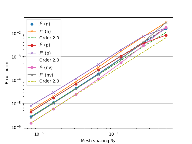
Fig. 16 Convergence test, showing \(l^2\) (RMS) and \(l^{\infty}\) (maximum) error for the evolving fields n (density), p (pressure) and nv (momentum). All fields are shown to converge at the expected second order accuracy.

Parallel diffusion

The parallel diffusion operator calculates \(\nabla_{||}\left[k\partial_||\left(f\right)\right]\)

const Field3D Div_par_K_Grad_par(const Field3D &k, const Field3D &f,
                                 bool bndry_flux=true);

This is done by calculating the flux \(k\partial_{||}\left(f\right)\) on cell boundaries using central differencing.

Advection in 3D

This operator calculates \(\nabla\cdot\left( n \mathbf{v} \right)\) where \(\mathbf{v}\) is a 3D vector. It is written in flux form by discretising the expression

\[\nabla\cdot\left( \mathbf{A} \right) = \frac{1}{J}\partial_i \left(J A^i\right)\]

Like the Div_par operator, a slope limiter is used to calculate the value of the field \(n\) on cell boundaries. By default this is the MC method, but this can be set as a template parameter.

template<typename CellEdges = MC>
const Field3D Div_f_v(const Field3D &n, const Vector3D &v, bool bndry_flux)

Slope limiters

Here limiters are implemented as slope limiters: The value of a given quantity is calculated at the faces of a cell based on the cell-centre values. Several slope limiters are defined in fv_ops.hxx:

• Upwind - First order upwinding, in which the left and right edges of the cell are the same as the centre (zero slope).

• Fromm - A second-order scheme which is a fixed weighted average of upwinding and central difference schemes.

• MinMod - This second order scheme switches between the upwind and downwind gradient, choosing the one with the smallest absolute value. If the gradients have different signs, as at a maximum or minimum, then the method reverts to first order upwinding (zero slope).

• MC (Monotonised Central) is a second order scheme which switches between central, upwind and downwind differencing in a similar way to MinMod. It has smaller dissipation than MinMod so is the default.

Staggered grids

By default, all quantities in BOUT++ are defined at cell centre, and all derivative methods map cell-centred quantities to cell centres. Switching on staggered grid support in BOUT.inp:

StaggerGrids = true

allows quantities to be defined on cell boundaries. Functions such as DDX now have to handle all possible combinations of input and output locations, in addition to the possible derivative methods.

Several things are not currently implemented, which probably should be:

• Only 3D fields currently have a cell location attribute. The location (cell centre etc) of 2D fields is ignored at the moment. The rationale for this is that 2D fields are assumed to be slowly-varying equilibrium quantities for which it won’t matter so much. Still, needs to be improved in future

• Twist-shift and X shifting still treat all quantities as cell-centred.

• No boundary condition functions yet account for cell location.

Currently, BOUT++ does not support values at cell corners; values can only be defined at cell centre, or at the lower X,Y, or Z boundaries. This is

Once staggered grids are enabled, two types of stencil are needed: those which map between the same cell location (e.g. cell-centred values to cell-centred values), and those which map to different locations (e.g. cell-centred to lower X).

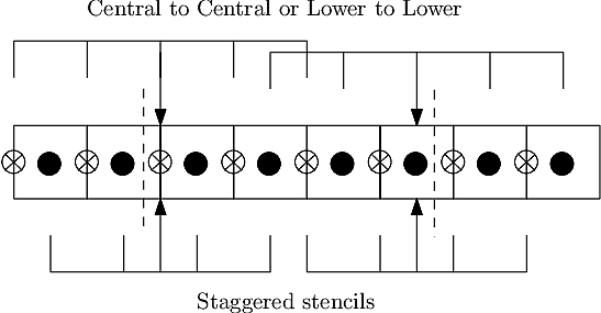
Fig. 17 Stencils with cell-centred (solid) and lower shifted values (open). Processor boundaries marked by vertical dashed line

Central differencing using 4-point stencil:

\[\begin{split}\begin{aligned} y &=& \left(9y_{-1/2} + 9y_{1/2} - y_{-3/2} - y_{3/2}\right) / 16 \\ {{\frac{\partial y}{\partial x}}} &=& \left( 27y_{1/2} - 27y_{-1/2} - y_{3/2} + y_{-3/2}\right) / 24\Delta x \\ \frac{\partial^2 y}{\partial x^2} &=& \left(y_{3/2} + y_{-3/2} - y_{1/2} - y_{-1/2}\right) / 2\Delta x^2\end{aligned}\end{split}\]

Input	Output	Actions
	Central stencil
CENTRE	XLOW	Lower staggered stencil
XLOW	CENTRE	Upper staggered stencil
XLOW	Any	Staggered stencil to CENTRE, then interpolate
CENTRE	Any	Central stencil, then interpolate
Any	Any	Interpolate to centre, use central stencil, then interpolate

Table: DDX actions depending on input and output locations. Uses first match.

Derivatives of the Fourier transform

By using the definition of the Fourier transformed, we have

\[F(x,y,\xi) = {\int_{-\infty}^{\infty} {f(x,y,z)\exp(-2\pi iz\xi)} \; \text{d} {z}}\]

this gives

(9)\[\begin{split}&{\int_{-\infty}^{\infty} {(\partial_zf[x,y,z])\exp(-2\pi iz\xi)} \; \text{d} {z}}\\ =& {\int_{-\infty}^{\infty} {\partial_z(f[x,y,z]\exp[-2\pi iz\xi])} \; \text{d} {z}} - {\int_{-\infty}^{\infty} {f(x,y,z)\partial_z\exp(-2\pi iz\xi)} \; \text{d} {z}}\\ =& (f[x,y,z]\exp[-2\pi iz\xi])\bigg|_{-\infty}^{\infty} - (-2\pi i\xi){\int_{-\infty}^{\infty} {f(x,y,z)\exp(-2\pi iz\xi)} \; \text{d} {z}}\\ =& 2\pi i\xi F(x,y,\xi)\end{split}\]

where we have used that \(f(x,y,\pm\infty)=0\) in order to have a well defined Fourier transform. This means that

\[\partial_z^n F(x,y,\xi) = (2\pi i \xi)^n F(x,y,\xi)\]

In our case, we are dealing with periodic boundary conditions. Strictly speaking, the Fourier transform does not exist in such cases, but it is possible to define a Fourier transform in the limit which in the end lead to the Fourier series [2] By discretising the spatial domain, it is no longer possible to represent the infinite amount of Fourier modes, but only \(N+1\) number of modes, where \(N\) is the number of points (this includes the modes with negative frequencies, and the zeroth offset mode). For the discrete Fourier transform, we have

(10)\[F(x,y)_{k} = \frac{1}{N}\sum_{Z=0}^{N-1}f(x,y)_{Z}\exp(\frac{-2\pi i k Z}{N})\]

where \(k\) is the mode number, \(N\) is the number of points in \(z\). If we call the sampling points of \(z\) for \(z_Z\), where \(Z = 0, 1 \ldots N-1\), we have that \(z_Z = Z \text{d}z\). As our domain goes from \([0, 2\pi[\), we have that (since we have one less line segment than point) \(\text{d}z (N-1) = L_z = 2\pi - \text{d}z\), which gives \(\text{d}z = \frac{2\pi}{N}\). Inserting this is equation ((10)) yields

\[F(x,y)_{k} = \frac{1}{N}\sum_{Z=0}^{N-1}f(x,y)_{Z}\exp( - i k Z\text{d}z) = \frac{1}{N}\sum_{Z=0}^{N-1}f(x,y)_{Z}\exp( - i k z_Z)\]

The discrete version of equation ((9)) thus gives

\[\partial_z^n F(x,y)_k = (i k)^n F(x,y)_k\]

[2]

For more detail see Bracewell, R. N. - The Fourier Transform and Its Applications 3rd Edition chapter 10