Nonlocal heat flux models#
Spitzer-Harm heat flux#
The Spitzer-Harm heat flux \(q_{SH}\) is calculated using
where \(n_e\) is the electron density in \(m^{-3}\), \(T_e\) is the electron temperature in eV, \(\kappa_0 = 13.58\), \(Z\) is the average ion charge. The resulting expression is in units of \(eV/m^2/s\).
The thermal collision time \(\tau_{ei,T} = \lambda_{ei,T} / v_{T}\) is calculated using the thermal mean free path and thermal velocity:
where it is assumed that \(n_i = n_e\), and the following are used:
Note: If comparing to online notes, \(\kappa_0\frac{Z+0.24}{Z+4.2} \simeq 3.2\), a different definition of collision time \(\tau_{ei}\) is used here, but the other factors are included so that the heat flux \(q_{SH}\) is the same here as in those notes.
SNB model#
The SNB model calculates a correction to the Spitzer-Harm heat flux, solving a diffusion equation for each of a set of energy groups with normalised energy \(\beta = E_g / eT_e\) where \(E_g\) is the energy of the group.
where \(\nabla_{||}\) is the divergence of a parallel flux, and \(\partial_{||}\) is a parallel gradient. \(U_g = W_g q_{SH}\) is the contribution to the Spitzer-Harm heat flux from a group:
The modified mean free paths for each group are:
From the quantities \(H_g\) for each group, the SNB heat flux is:
In flud models we actually want the divergence of the heat flux, rather than the heat flux itself. We therefore rearrange to get:
and so calculate the divergence of the heat flux as:
The Helmholtz type equation along the magnetic field is solved using a tridiagonal solver. The parallel divergence term is currently split into a second derivative term, and a first derivative correction:
Using the SNB model#
To use the SNB model, first include the header:
#include <bout/snb.hxx>
then create an instance:
HeatFluxSNB snb;
By default this will use options in a section called “snb”, but if
needed a different Options& section can be given to the constructor:
HeatFluxSNB snb(Options::root()["mysnb"]);
The options are listed in table Table 17.
Name |
Meaning |
Default value |
|---|---|---|
|
Maximum energy group to consider (multiple of eT) Number of energy groups Scaling down the electron-electron mean free path |
10 40 2 |
The divergence of the heat flux can then be calculated:
Field3D Div_q = snb.divHeatFlux(Te, Ne);
where Te is the temperature in eV, and Ne is the electron density in \(m^{-3}\).
The result is in eV per \(m^3\) per second, so multiplying by \(e=1.602\times 10^{-19}\) will give
Watts per cubic meter.
To compare to the Spitzer-Harm result, pass in a pointer to a
Field3D as the third argument. This field will be set to the
Spitzer-Harm value:
Field3D Div_q_SH;
Field3D Div_q = snb.divHeatFlux(Te, Ne, &Div_q_SH);
This is used in the examples discussed below.
Example: Linear perturbation#
The examples/conduction-snb example calculates the heat flux for a
given density and temperature profile, comparing the SNB and
Spitzer-Harm fluxes. The sinusoidal.py case uses a periodic
domain of length 1 meter and a small (0.01eV) perturbation to the
temperature. The temperature is varied from 1eV to 1keV, so that the
mean free path varies. This is done for different SNB settings,
changing the number of groups and the maximum \(\beta\):
$ python sinusoid.py
This should output a file snb-sinusoidal.png and display the results,
shown in figure Fig. 16.
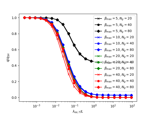
Fig. 16 The ratio of SNB heat flux to Spitzer-Harm heat flux, as a function of electron mean free path divided by temperature perturbation wavelength. Note that the difference between SNB and Spitzer-Harm becomes significant (20%) when the mean free path is just 1% of the wavelength.#
Example: Nonlinear heat flux#
A nonlinear test is also included in examples/conduction-snb, a step function in temperature
from around 200eV to 950eV over a distance of around 0.1mm, at an electron density of 5e26 per cubic meter:
$ python step.py
This should output a file snb-step.png, shown in figure Fig. 17.
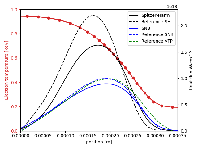
Fig. 17 Temperature profile and heat flux calculated using Spitzer-Harm and the SNB model, for a temperature step profile, at a density of 5e26 per cubic meter. Note the reduction in peak heat flux (flux limit) and higher flux in the cold region (preheat) with the SNB model.#