Variable initialisation#

Variables in BOUT++ are not initialised automatically, but must be explicitly given a value. For example the following code declares a Field3D variable then attempts to access a particular element:

Field3D f;    // Declare a variable
f(0,0,0) = 1.0;  // Error!

This results in an error because the data array to store values in f has not been allocated. Allocating data can be done in several ways:

Initialise with a value:
```
Field3D f = 0.0; // Allocates memory, fills with zeros
f(0,0,0) = 1.0; // ok
```
This cannot be done at a global scope, since it requires the mesh to already exist and have a defined size.
Set to a scalar value:
```
Field3D f;
f = 0.0; // Allocates memory, fills with zeros
f(0,0,0) = 1.0; // ok
```
Note that setting a field equal to another field has the effect of making both fields share the same underlying data. This behaviour is similar to how NumPy arrays behave in Python.
```
Field3D g = 0.0;  // Allocates memory, fills with zeros
Field3D f = g; // f now shares memory with g

f(0,0,0) = 1.0; // g also modified
```
To ensure that a field has a unique underlying memory array call the Field3D::allocate() method before writing to individual indices.

Use Field3D::allocate() to allocate memory:

Field3D f;
f.allocate(); // Allocates memory, values undefined
f(0,0,0) = 1.0; // ok

In a BOUT++ simulation some variables are typically evolved in time. The initialisation of these variables is handled by the time integration solver.

Initialisation of time evolved variables#

Each variable being evolved has its own section, with the same name as the output data. For example, the high-\(\beta\) model has variables “P”, “jpar”, and “U”, and so has sections [P], [jpar], [U] (names are case sensitive).

Expressions#

The recommended way to initialise a variable is to use the function option for each variable:

[p]
function = 1 + gauss(x-0.5)*gauss(y)*sin(z)

This evaluates an analytic expression to initialise the \(P\) variable. Expressions can include the usual operators (+,-,*,/), including ^ for exponents. The following values are also already defined:

Table 1 Initialisation expression values#
Name	Description
x	\(x\) position between \(0\) and \(1\)
y	\(y\) angle-like position, definition depends on topology of grid
z	\(z\) position between \(0\) and \(2\pi\) (excluding the last point)
pi π	\(3.1415\ldots\)

By default, \(x\) is defined as (i+0.5) / (nx - 2*MXG), where MXG is the width of the boundary region (by default 2) and i is the x-index value on the grid excluding boundary points. Hence \(x\) actually goes from 0 on the boundary to the left of the leftmost point to 1 on the rightmost point boundary to the right of the rightmost grid point.

Note

The previous default (prior to v3.0), was for \(x\) to be defined as (i + MXG) / (nx - 2*MXG). Then \(x\) actually goes from 0 on the leftmost boundary point to (nx-1)/(nx-4) on the rightmost boundary point. To revert to the old behaviour, set

[mesh]
symmetricGlobalX = false

For slab-like or limiter-like geometries with no branch cuts, \(y\) is an angular coordinate between \(0\) and \(2\pi\), defined as (j + 0.5) / ny where j is the y-index value on the grid excluding boundary points. Hence \(y\) actually goes from \(0\) on the boundary to the left of the leftmost point to \(2\pi\) on the rightmost point boundary to the right of the rightmost grid point.

For tokamak geometries, \(y\) is an angular coordinate which goes between \(0\) and \(2\pi\) in the core region. In a single-null geometry or before the upper divertor in a double-null, \(y\) is defined as 2*pi*(j - 0.5 - jyseps1_1) / ny_core, where ny_core = (jyseps2_1 - jyseps1_1) + (jyseps2_2 - jyseps1_2) is the number of points in the core region. After the upper divertor in a double-null, \(y\) is defined as 2*pi*(j - 0.5 - jyseps1_1 - (jyseps1_2 - jyseps2_1)) / ny_core. So \(y\) has values less than \(0\) in the lower, inner divertor leg and greater than \(2\pi\) in the lower, outer divertor leg. In the upper, inner divertor leg of a double-null geometry, \(y\) increases smoothly from the value it had in the inner-core/inner-SOL, jumping at the location of the target so that in the upper, outer divertor leg it joins smoothly to the outer-core/outer-SOL.

Note

The previous default (prior to v3.0), was for \(y\) to be defined as j_core / ny_core where j_core is the grid index excluding boundary points and points in any divertor legs (j_core = 0 in the lower, inner divertor leg, j_core = jyseps2_1 - jyseps1_1 in the upper divertor legs if present, j_core = ny_core in the lower, outer divertor leg). To revert to the old behaviour, set

[mesh]
symmetricGlobalY = false

\(z\) is defined as k / nz where k is the z-index value on the grid. So \(z\) is 0 at the first grid point, and would be \(2\pi\) at the next point after the last grid point.

If a variable is at a staggered grid location CELL_XLOW, CELL_YLOW, or CELL_ZLOW, the values of \(x\), \(y\), or \(z\) respectively will take into account the half-grid-point shift.

By default the expressions are evaluated in a field-aligned coordinate system, i.e. if you are using the [mesh] option paralleltransform = shifted, the input f will have f = fromFieldAligned(f) applied before being returned. To switch off this behaviour and evaluate the input expressions in coordinates with orthogonal x-z (i.e. toroidal \(\{\psi,\theta,\phi\}\) coordinates when using paralleltransform = shifted), set in BOUT.inp

[input]
transform_from_field_aligned = false

The functions in Table 2 are also available in expressions.

Table 2 Initialisation expression functions#
Name	Description
`abs(x)`	Absolute value \(\|x\|\)
`asin(x)`, `acos(x)`, `atan(x)`, `atan(y,x)`	Inverse trigonometric functions
`ballooning(x)`	Ballooning transform ((1), Fig. 4)
`ballooning(x,n)`	Ballooning transform, using \(n\) terms (default 3)
`cos(x)`	Cosine
`cosh(x)`	Hyperbolic cosine
`exp(x)`	Exponential
`tanh(x)`	Hyperbolic tangent
`gauss(x)`	Gaussian \(\exp(-x^2/2) / \sqrt{2\pi}\)
`gauss(x, w)`	Gaussian \(\exp[-x^2/(2w^2)] / (w\sqrt{2\pi})\)
`H(x)`	Heaviside function: \(1\) if \(x > 0\) otherwise \(0\)
`log(x)`	Natural logarithm
`max(x,y,...)`	Maximum (variable arguments)
`min(x,y,...)`	Minimum (variable arguments)
`clamp(value, low, high)`	If value < low, return low; If value > high, return high; otherwise return value
`mixmode(x)`	A mixture of Fourier modes
`mixmode(x, seed)`	seed determines random phase (default 0.5)
`power(x,y)`	Exponent \(x^y\)
`sin(x)`	Sine
`sinh(x)`	Hyperbolic sine
`sqrt(x)`	\(\sqrt{x}\)
`tan(x)`	Tangent
`erf(x)`	The error function
`TanhHat(x, width, centre, steepness)`	The hat function \(\frac{1}{2}(\tanh[s (x-[c-\frac{w}{2}])]\) \(- \tanh[s (x-[c+\frac{w}{2}])] )\)
`fmod(x)`	The modulo operator, returns floating point remainder

In addition there are some special functions which enable control flow

Table 3 Control flow and special functions#
Name	Description
`where(expr, gt0, lt0)`	If the first `expr` evaluates to a value greater than zero then the second expression `gt0` is evaluated. Otherwise the last expression `lt0`
`sum(symbol, count, expr)`	Evaluate expression `expr` `count` times, and sum the result. Each time the symbol is incremented from 0 to `count`-1. The value of the symbol is accessed by putting it in braces `{}`. Example: `sum(i, 3, {i}^2)` is `0^2 + 1^2 + 2^2`
`[var = value,...](expr)`	Define a new scope with variables whose value can be accessed using braces `{}`. The `value` each variable `var` is set to can be an expression, and is evaluated before the `expr` expression. Example: `[n=2]( {n}^{n} )` is `2^2`.

For field-aligned tokamak simulations, the Y direction is along the field and in the core this will have a discontinuity at the twist-shift location where field-lines are matched onto each other. To handle this, the ballooning function applies a truncated Ballooning transformation to construct a smooth initial perturbation:

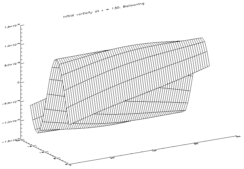
(1)#\[U_0^{balloon} = \sum_{i=-N}^N F(x)G(y + 2\pi i)H(z + q2\pi i)\]

Fig. 4 Initial profiles in twist-shifted grid. **Left**: Without ballooning transform, showing discontinuity at the matching location **Right**: with ballooning transform#

There is an example code test-ballooning which compares methods of setting initial conditions with the ballooning transform.

The mixmode(x) function is a mixture of Fourier modes of the form:

\[\mathrm{mixmode}(x) = \sum_{i=1}^{14} \frac{1}{(1 + |i-4|)^2}\cos[ix + \phi(i, \mathrm{seed})]\]

where \(\phi\) is a random phase between \(-\pi\) and \(+\pi\), which depends on the seed. The factor in front of each term is chosen so that the 4th harmonic (\(i=4\)) has the highest amplitude. This is useful mainly for initialising turbulence simulations, where a mixture of mode numbers is desired.

Context variables and scope#

Expressions can use a form of local variables, by using []() to define new scopes:

var = [a = 2,
       b = 3]( {a} + {b}^{a} )

Where here the braces {} refer to context variables, to distinguish them from variables in the options which have no braces. One application of these is a (modest) performance improvement: If {a} is a large expression then in the above example it would only be evaluated once, the value stored as {a} and used twice in the expression.

Passing data into expressions#

A second application of context variables is that they can be set by the calling C++ code, providing a way for data to be passed from BOUT++ into these expressions. The evaluation of expressions is currently not very efficient, but this provides a very flexible way for the input options to modify simulation behaviour.

This can be done by first parsing an expression and then passing values to generate in the Context object.

Field3D shear = ...; // Value calculated in BOUT++

FieldFactory factory(mesh);
auto gen = factory->parse("model:viscosity");

Field3D viscosity;
viscosity.allocate();

BOUT_FOR(i, viscosity.region("RGN_ALL")) {
  viscosity[i] = gen->generate(bout::generator::Context(i, CELL_CENTRE, mesh, 0.0)
                                 .set("shear", shear[i]));
}

Note that the Context constructor takes the index, the cell location (e.g. staggered), a mesh, and then the time (set to 0.0 here). Additional variables can be set, “shear” in this case. In the input options file (or command line) the viscosity could now be a function of {shear}

[model]
viscosity = 1 + {shear}

Defining functions in input options#

Defining context variables in a new scope can be used to define and call functions, as in the above example viscosity is a function of {shear}. For example we could define a cosh function using

mycosh = 0.5 * (exp({arg}) + exp(-{arg}))

which uses {arg} as the input value. We could then call this function:

result = [arg = x*2](mycosh)

Recursive functions#

By default recursive expressions are not allowed in the input options, and a ParseException will be thrown if circular dependencies occur. Recursive functions can however be enabled by setting input:max_recursion_depth != 0 e.g.:

[input]
max_recursion_depth = 10  # 0 = none, -1 = unlimited

By putting a limit on the depth, expressions should (eventually) terminate or fail with a BoutException, rather than entering an infinite loop. To remove this restriction max_recursion_depth can be set to -1 to allow arbitrary recursion (limited by stack, memory sizes).

If recursion is allowed, then the where special function and Context scopes can be (ab)used to define quite general functions. For example the Fibonnacci sequence 1,1,2,3,5,8,... can be generated:

fib = where({n} - 2.5,
            [n={n}-1](fib) + [n={n}-2](fib),
            1)

so if n = 1 or 2 then fib = 1, but if n = 3 or above then recursion is used.

Note: Use of this facility in general is not encouraged, as it can easily lead to very inefficient and hard to understand code. It is here because occasionally it might be necessary, and because making the input language Turing complete was irresistible.

Initalising variables with the `FieldFactory` class#

This class provides a way to generate a field with a specified form. For example to create a variable var from options we could write

FieldFactory f(mesh);
Field2D var = f.create2D("var");

This will look for an option called “var”, and use that expression to initialise the variable var. This could then be set in the BOUT.inp file or on the command line.

var = gauss(x-0.5,0.2)*gauss(y)*sin(3*z)

To do this, FieldFactory implements a recursive descent parser to turn a string containing something like "gauss(x-0.5,0.2)*gauss(y)*sin(3*z)" into values in a Field3D or Field2D object. Examples are given in the test-fieldfactory example:

FieldFactory f(mesh);
Field2D b = f.create2D("1 - x");
Field3D d = f.create3D("gauss(x-0.5,0.2)*gauss(y)*sin(z)");

This is done by creating a tree of FieldGenerator objects which then generate the field values:

class FieldGenerator {
 public:
  virtual ~FieldGenerator() { }
  virtual FieldGeneratorPtr clone(const list<FieldGeneratorPtr> args) {return NULL;}
  virtual BoutReal generate(const bout::generator::Context& ctx) = 0;
};

where FieldGeneratorPtr is an alias for std::shared_ptr, a shared pointer to a FieldGenerator. The Context input to generate is an object containing values which can be used in expressions, in particular x, y, z and t coordinates. Additional values can be stored in the Context object, allowing data from BOUT++ to be used in expressions. There are also ways to manipulate Context objects for more complex expressions and functions, see below for details.

All classes inheriting from FieldGenerator must implement a FieldGenerator::generate() function, which returns the value at the given (x,y,z,t) position. Classes should also implement a FieldGenerator::clone() function, which takes a list of arguments and creates a new instance of its class. This takes as input a list of other FieldGenerator objects, allowing a variable number of arguments.

The simplest generator is a fixed numerical value, which is represented by a FieldValue object:

class FieldValue : public FieldGenerator {
 public:
  FieldValue(BoutReal val) : value(val) {}
  BoutReal generate(const bout::generator::Context&) override { return value; }
 private:
  BoutReal value;
};

Adding a new function#

To add a new function to the FieldFactory, a new FieldGenerator class must be defined. Here we will use the example of the sinh function, implemented using a class FieldSinh. This takes a single argument as input, but FieldPI takes no arguments, and FieldGaussian takes either one or two. Study these after reading this to see how these are handled.

First, edit src/field/fieldgenerators.hxx and add a class definition:

class FieldSinh : public FieldGenerator {
 public:
  FieldSinh(FieldGeneratorPtr g) : gen(g) {}

  FieldGeneratorPtr clone(const list<FieldGenerator*> args) override;
  BoutReal generate(const bout::generator::Context& ctx) override;
 private:
  FieldGeneratorPtr gen;
};

The gen member is used to store the input argument. The constructor takes a single input, the FieldGenerator argument to the sinh function, which is stored in the member gen .

Next edit src/field/fieldgenerators.cxx and add the implementation of the clone and generate functions:

FieldGeneratorPtr FieldSinh::clone(const list<FieldGeneratorPtr> args) {
  if (args.size() != 1) {
    throw ParseException("Incorrect number of arguments to sinh function. Expecting 1, got %d", args.size());
  }

  return std::make_shared<FieldSinh>(args.front());
}

BoutReal FieldSinh::generate(const bout::generator::Context& ctx) {
  return sinh(gen->generate(ctx));
}

The clone function first checks the number of arguments using args.size() . This is used in FieldGaussian to handle different numbers of input, but in this case we throw a ParseException if the number of inputs isn’t one. clone then creates a new FieldSinh object, passing the first argument ( args.front() ) to the constructor (which then gets stored in the gen member variable). Note that std::make_shared is used to make a shared pointer.

The generate function for sinh just gets the value of the input by calling gen->generate(ctx) with the input Context object ctx, calculates sinh of it and returns the result.

The clone function means that the parsing code can make copies of any FieldGenerator class if it’s given a single instance to start with. The final step is therefore to give the FieldFactory class an instance of this new generator. Edit the FieldFactory constructor FieldFactory::FieldFactory() in src/field/field_factory.cxx and add the line:

addGenerator("sinh", std::make_shared<FieldSinh>(nullptr));

That’s it! This line associates the string "sinh" with a FieldGenerator . Even though FieldFactory doesn’t know what type of FieldGenerator it is, it can make more copies by calling the clone member function. This is a useful technique for polymorphic objects in C++ called the “Virtual Constructor” idiom.

Parser internals#

The basic expression parser is defined in include/bout/sys/expressionparser.hxx and the code in src/sys/expressionparser.cxx. The FieldFactory adds the function in table Table 2 on top of this basic functionality, and also uses Options to resolve unknown symbols to Options.

When a FieldGenerator is added using the addGenerator function, it is entered into a std::map which maps strings to FieldGenerator objects (include/bout/sys/expressionparser.hxx):

std::map<std::string, FieldGeneratorPtr> gen;

Parsing a string into a tree of FieldGenerator objects is done by a first splitting the string up into separate tokens like operators like ’*’, brackets ’(’, names like ’sinh’ and so on (Lexical analysis), then recognising patterns in the stream of tokens (Parsing). Recognising tokens is done in src/sys/expressionparser.cxx:

char ExpressionParser::LexInfo::nextToken() {
 ...

This returns the next token, and setting the variable char curtok to the same value. This can be one of:

-1 if the next token is a number. The variable BoutReal curval is set to the value of the token
-2 for a symbol (e.g. “sinh”, “x” or “pi”). This includes anything which starts with a letter, and contains only letters, numbers, and underscores. The string is stored in the variable string curident
-3 for a Context parameter which appeared surrounded by braces {}.
0 to mean end of input
The character if none of the above. Since letters and numbers are taken care of (see above), this includes brackets and operators like ’+’ and ’-’.

The parsing stage turns these tokens into a tree of FieldGenerator objects, starting with the parse() function:

FieldGenerator* FieldFactory::parse(const string &input) {
   ...

which puts the input string into a stream so that nextToken() can use it, then calls the parseExpression() function to do the actual parsing:

FieldGenerator* FieldFactory::parseExpression() {
   ...

This breaks down expressions in stages, starting with writing every expression as:

expression := primary [ op primary ]

i.e. a primary expression, and optionally an operator and another primary expression. Primary expressions are handled by the parsePrimary() function, so first parsePrimary() is called, and then parseBinOpRHS which checks if there is an operator, and if so calls parsePrimary() to parse it. This code also takes care of operator precedence by keeping track of the precedence of the current operator. Primary expressions are then further broken down and can consist of either a number, a name (identifier), a minus sign and a primary expression, or brackets around an expression:

primary := number
        := identifier
        := '-' primary
        := '(' expression ')'
        := '[' expression ']'

The minus sign case is needed to handle the unary minus e.g. "-x" . Identifiers are handled in parseIdentifierExpr() which handles either variable names, or functions

identifier := name
           := name '(' expression [ ',' expression [ ',' ... ] ] ')'

i.e. a name, optionally followed by brackets containing one or more expressions separated by commas. names without brackets are treated the same as those with empty brackets, so "x" is the same as "x()". A list of inputs (list<FieldGeneratorPtr> args; ) is created, the gen map is searched to find the FieldGenerator object corresponding to the name, and the list of inputs is passed to the object’s clone function.