BOUT++ physics models#
Once you have tried some example codes, and generally got the hang of running BOUT++ and analysing the results, there will probably come a time when you want to change the equations being solved. This section demonstrates how a BOUT++ physics model is put together. It assumes you have a working knowledge of C or C++, but you don’t need to be an expert - most of the messy code is hidden away from the physics model. There are several good books on C and C++, but I’d recommend online tutorials over books because there are a lot more of them, they’re quicker to scan through, and they’re cheaper.
Many of the examples which come with BOUT++ are physics models, and
can be used as a starting point. Some relatively simple examples are
blob2d (2D plasma filament/blob propagation),
hasegawa-wakatani (2D turbulence), finite-volume/fluid (1D
compressible fluid) and gas-compress (up to 3D compressible
fluid). Some of the integrated tests (under tests/integrated) use
either physics models (e.g. test-delp2 and
test-drift-instability), or define their own main function
(e.g. test-io and test-cyclic).
Building Physics Models#
After building the library (see Configuring BOUT++), you can build a physics model in several different ways.
For the bundled examples, perhaps the easiest is to build it directly
in the build directory. For example, to build the conduction
example:
$ cmake --build build --target conduction
(assuming that your build directory is called build!) which will
build the executable in build/examples/conduction.
You can also cd into that directory and build it there:
$ cd build/examples/conduction
$ make
(Note for advanced users that this won’t work if you’ve used the
Ninja CMake generator).
Either of these two methods will actually build the entire BOUT++ library if necessary, which can be especially useful when developing.
Using CMake with your physics model#
You can write a CMake configuration file (CMakeLists.txt) for your
physics model in only four lines:
project(blob2d LANGUAGES CXX)
find_package(bout++ REQUIRED)
add_executable(blob2d blob2d.cxx)
target_link_libraries(blob2d PRIVATE bout++::bout++)
You just need to give CMake the location where you built or installed
BOUT++ via the bout++_DIR variable:
$ cmake . -B build -Dbout++_DIR=/path/to/built/BOUT++
If you want to modify BOUT++ along with developing your model, you may
instead wish to place the BOUT++ as a subdirectory of your model and
use add_subdirectory instead of find_package above:
project(blob2d LANGUAGES CXX)
add_subdirectory(BOUT++/source)
add_executable(blob2d blob2d.cxx)
target_link_libraries(blob2d PRIVATE bout++::bout++)
where BOUT++/source is the subdirectory containing the BOUT++
source. Doing this has the advantage that any changes you make to
BOUT++ source files will trigger a rebuild of both the BOUT++ library
and your model when you next build your code.
Heat conduction#
The conduction example solves 1D heat conduction
The source code to solve this is in conduction.cxx, which we show here:
 6#include <bout/physicsmodel.hxx>
 7
 8class Conduction : public PhysicsModel {
 9private:
10  Field3D T; // Evolving temperature equation only
11
12  BoutReal chi; // Parallel conduction coefficient
13
14protected:
15  // This is called once at the start
16  int init(bool UNUSED(restarting)) override {
17
18    // Get the options
19    auto& options = Options::root()["conduction"];
20
21    // Read from BOUT.inp, setting default to 1.0
22    // The doc() provides some documentation in BOUT.settings
23    chi = options["chi"].doc("Conduction coefficient").withDefault(1.0);
24
25    // Tell BOUT++ to solve T
26    SOLVE_FOR(T);
27
28    return 0;
29  }
30
31  int rhs(BoutReal UNUSED(time)) override {
32    mesh->communicate(T); // Communicate guard cells
33
34    ddt(T) =
35        Div_par_K_Grad_par(chi, T); // Parallel diffusion Div_{||}( chi * Grad_{||}(T) )
36
37    return 0;
38  }
39};
40
41BOUTMAIN(Conduction);
Let’s go through it line-by-line. First, we include the header that
defines the PhysicsModel class:
#include <bout/physicsmodel.hxx>
This also brings in the header files that we need for the rest of the
code. Next, we need to define a new class, Conduction, that
inherits from PhysicsModel (line 8):
class Conduction : public PhysicsModel {
The PhysicsModel contains both the physical variables we want to
evolve, like the temperature:
Field3D T; // Evolving temperature equation only
as well as any physical or numerical coefficients. In this case, we
only have the parallel conduction coefficient, chi:
BoutReal chi; // Parallel conduction coefficient
A Field3D represents a 3D scalar quantity, while a BoutReal
represents a single number. See the later section on
Variables for more information.
After declaring our model variables, we need to define two functions:
an initialisation function, init, that is called to set up the
simulation and specify which variables are evolving in time; and a
“right-hand side” function, rhs, that calculates the time
derivatives of our evolving variables. These are defined in lines 18
and 21 respectively above:
int init(bool restarting) override {
...
}
int rhs(BoutReal time) override {
...
}
PhysicsModel::init takes as input a bool (true or false)
that tells it whether or not the model is being restarted, which can
be useful if something only needs to be done once before the
simulation starts properly. The simulation (physical) time is passed
to PhyiscsModel::rhs as a BoutReal.
The override keyword is just to let the compiler know we’re
overriding a method in the base class and is not important to
understand.
Initialisation#
During initialisation (the init function), the conduction example
first reads an option (lines 21 and 24) from the input settings file
(data/BOUT.inp by default):
auto& options = Options::root()["conduction"];

OPTION(options, chi, 1.0);
This first gets a section called “conduction”, then requests an option called “chi” inside this section. If this setting is not found, then the default value of 1.0 will be used. To set this value the BOUT.inp file contains:
[conduction]
chi = 1.0
which defines a section called “conduction”, and within that section a variable called “chi”. This value can also be overridden by specifying the setting on the command line:
$ ./conduction conduction:chi=2
where conduction:chi means the variable “chi” in the section
“conduction”. When this option is read, a message is printed to the
BOUT.log files, giving the value used and the source of that value:
Option conduction:chi = 1 (data/BOUT.inp)
For more information on options and input files, see
BOUT++ options, as well as the documentation for the Options
class.
After reading the chi option, the init method then specifies which
variables to evolve using the SOLVE_FOR macro:
// Tell BOUT++ to solve T
SOLVE_FOR(T);
This tells the BOUT++ time integration solver to set the variable
T using values from the input settings. It looks in a section with
the same name as the variable (T here) for variables “scale” and
“function”:
[T] # Settings for the T variable

scale = 1.0  # Size of the initial perturbation
function = gauss(y-pi, 0.2)  # The form of the initial perturbation. y from 0 to 2*pi
The function is evaluated using expressions which can involve x,y and z coordinates. More details are given in section Initialisation of time evolved variables.
Finally an error code is returned, here 0 indicates no error. If
init returns non-zero then the simulation will stop.
Time evolution#
During time evolution, the time integration method (ODE integrator)
calculates the system state (here T) at a give time. It then calls
the PhysicsModel::rhs function, which should calculate the time
derivative of all the evolving variables. In this case the job of the
rhs function is to calculate ddt(T), the partial
derivative of the variable T with respect to time, given the value
of T:
\[\frac{\partial T}{\partial t} = \nabla_{||}(\chi\partial_{||} T)\]
The first thing the rhs function function does is communicate the
guard (halo) cells using Mesh::communicate on line 33:
mesh->communicate(T);
This is because BOUT++ does not (generally) do communications, but
leaves it up to the user to decide when the most efficient or
convenient time to do them is. Before we can take derivatives of a
variable (here T), the values of the function must be known in the
boundaries and guard cells, which requires communication between
processors. By default the values in the guard cells are set to
NaN, so if they are accidentally used without first communicating
then the code should crash fairly quickly with a non-finite number
error.
Once the guard cells have been communicated, we calculate the right hand side (RHS) of the equation above (line 35):
ddt(T) = Div_par_K_Grad_par(chi, T);
The function Div_par_K_Grad_par is a function in the BOUT++ library
which calculates the divergence in the parallel (y) direction of a
constant multiplied by the gradient of a function in the parallel
direction.
As with the init code, a non-zero return value indicates an error
and will stop the simulation.
Running the model#
The very last thing we need to do in our physics model is to define a
main function. Here, we do it with the BOUTMAIN macro:
BOUTMAIN(Conduction);
You can define your own main() function, but for most cases this
is enough. The macro expands to something like:
int main(int argc, char **argv) {
  BoutInitialise(argc, argv); // Initialise BOUT++

  Conduction *model = new Conduction(); // Create a model

  Solver *solver = Solver::create(); // Create a solver
  solver->setModel(model); // Specify the model to solve
  solver->addMonitor(bout_monitor); // Monitor the solver

  solver->solve(); // Run the solver

  delete model;
  delete solver;
  BoutFinalise(); // Finished with BOUT++
  return 0;
}
This initialises the main BOUT++ library, creates the PhysicsModel
and Solver, runs the solver, and finally cleans up the model, solver
and library.
Magnetohydrodynamics (MHD)#
When going through this section, it may help to refer to the finished
code, which is given in the file mhd.cxx in the BOUT++ examples
directory under orszag-tang. The equations to be solved are:
As in the heat conduction example,
a class is created which inherits from PhysicsModel and defines
init and rhs functions:
class MHD : public PhysicsModel {
  private:
  int init(bool restarting) override {
    ...
  }
  int rhs(BoutReal t) override {
    ...
  }
};
The init function is called once at the start of the simulation,
and should set up the problem, specifying which variables are to be
evolved. The argument restarting is false the first time a
problem is run, and true if loading the state from a restart file.
The rhs function is called every time-step, and should calculate
the time-derivatives for a given state. In both cases returning
non-zero tells BOUT++ that an error occurred.
Variables#
We need to define the variables to evolve as member variables (so they
can be used in init and rhs).
For ideal MHD, we need two 3D scalar fields density \(\rho\) and pressure \(p\), and two 3D vector fields velocity \(v\), and magnetic field \(B\):
class MHD : public PhysicsModel {
  private:
  Field3D rho, p; // 3D scalar fields
  Vector3D v, B;  // 3D vector fields
  ...
};
Scalar and vector fields behave much as you would expect: Field3D
objects can be added, subtracted, multiplied and divided, so the
following examples are all valid operations:
Field3D a, b, c;
BoutReal r;

a = b + c; a = b - c;
a = b * c; a = r * b;
a = b / c; a = b / r; a = r / b;
Similarly, vector objects can be added/subtracted from each other, multiplied/divided by scalar fields and real numbers, for example:
Vector3D a, b, c;
Field3D f;
BoutReal r;

a = b + c; a = b - c;
a = b * f; a = b * r;
a = b / f; a = b / r;
In addition the dot and cross products are represented by * and
\(\wedge\) symbols:
Vector3D a, b, c;
Field3D f;

f = a * b // Dot-product
a = b ^ c // Cross-product
For both scalar and vector field operations, so long as the result of an operation is of the correct type, the usual C/C++ shorthand notation can be used:
Field3D a, b;
Vector3D v, w;

a += b; v *= a; v -= w; v ^= w; // valid
v *= w; // NOT valid: result of dot-product is a scalar
Note: The operator precedence for \(\wedge\) is lower than
+, * and / so it is recommended to surround a ^ b with
braces.
Evolution equations#
At this point we can tell BOUT++ which variables to evolve, and where
the state and time-derivatives will be stored. This is done using the
bout_solve(variable, name) function in
your physics model init:
int init(bool restarting) {
  bout_solve(rho, "density");
  bout_solve(p,   "pressure");
  v.covariant = true; // evolve covariant components
  bout_solve(v,   "v");
  B.covariant = false; // evolve contravariant components
  bout_solve(B,   "B");

  return 0;
}
The name given to this function will be used in the output and restart data files. These will be automatically read and written depending on input options (see BOUT++ options). Input options based on these names are also used to initialise the variables.
You can add a description of the variable which will be saved as an
attribute in the output files by adding a third argument to
bout_solve() e.g.:
bout_solve(rho, "density", "electron density");
bout_solve(B, "B", "total magnetic field strength");
If the name of the variable in the output file is the same as the
variable name, you can use a shorthand macro. In this case, we could use
this shorthand for v and B:
SOLVE_FOR(v);
SOLVE_FOR(B);
To make this even shorter, multiple fields can be passed to
SOLVE_FOR (up to 10 at the time of writing). We can also use
macros SOLVE_FOR2, SOLVE_FOR3, …, SOLVE_FOR6 which are used in
many models. Our initialisation code becomes:
int init(bool restarting) override {
  ...
  bout_solve(rho, "density");
  bout_solve(p,   "pressure");
  v.covariant = true; // evolve covariant components
  B.covariant = false; // evolve contravariant components
  SOLVE_FOR(v, B);
  ...
  return 0;
}
Vector quantities can be stored in either covariant or contravariant
form. The value of the Vector3D::covariant property when
PhysicsModel::bout_solve (or SOLVE_FOR) is called is the form
which is evolved in time and saved to the output file.
The equations to be solved can now be written in the rhs
function. The value passed to the function (BoutReal t) is the
simulation time - only needed if your equations contain time-dependent
sources or similar terms. To refer to the time-derivative of a
variable var, use ddt(var). The ideal MHD equations can be
written as:
int rhs(BoutReal t) override {
  ddt(rho) = -V_dot_Grad(v, rho) - rho*Div(v);
  ddt(p) = -V_dot_Grad(v, p) - g*p*Div(v);
  ddt(v) = -V_dot_Grad(v, v) + ( (Curl(B)^B) - Grad(p) ) / rho;
  ddt(B) = Curl(v^B);
}
Where the differential operators vector = Grad(scalar),
scalar = Div(vector), and vector = Curl(vector) are
used. For the density and pressure equations, the
\(\mathbf{v}\cdot\nabla\rho\) term could be written as
v*Grad(rho), but this would then use central differencing in the
Grad operator. Instead, the function V_dot_Grad uses upwinding
methods for these advection terms. In addition, the Grad function
will not operate on vector objects (since result is neither scalar nor
vector), so the \(\mathbf{v}\cdot\nabla\mathbf{v}\) term CANNOT be
written as v*Grad(v).
Input options#
Note that in the above equations the extra parameter g has been
used for the ratio of specific heats. To enable this to be set in the
input options file (see BOUT++ options), we use the Options
object in the initialisation function:
class MHD : public PhysicsModel {
  private:
  BoutReal gamma;

  int init(bool restarting) override {
    auto& globalOptions = Options::root();
    auto& options = globalOptions["mhd"];

    OPTION(options, g, 5.0 / 3.0);
    ...
This specifies that an option called “g” in a section called “mhd”
should be put into the variable g. If the option could not be
found, or was of the wrong type, the variable should be set to a
default value of \(5/3\). The value used will be printed to the
output file, so if g is not set in the input file the following
line will appear:
Option mhd:g = 1.66667 (default)
This function can be used to get integers and booleans. To get
strings, there is the function (char* options.getString(section,
name). To separate options specific to the physics model, these
options should be put in a separate section, for example here the
“mhd” section has been specified.
Most of the time, the name of the variable (e.g. g) will be the
same as the identifier in the options file (“g”). In this case, there
is the macro:
OPTION(options, g, 5.0/3.0);
which is equivalent to:
g = options["g"].withDefault( 5.0/3.0 );
See BOUT++ options for more details of how to use the input options.
Communication#
If you plan to run BOUT++ on more than one processor, any operations
involving derivatives will require knowledge of data stored on other
processors. To handle the necessary parallel communication, there is
the mesh->communicate function. This takes care
of where the data needs to go to/from, and only needs to be told which
variables to transfer.
If you only need to communicate a small number (up to 5 currently) of
variables then just call the Mesh::communicate function directly.
For the MHD code, we need to communicate the variables rho,p,v,B
at the beginning of the PhysicsModel::rhs function before any
derivatives are calculated:
int rhs(BoutReal t) override {
  mesh->communicate(rho, p, v, B);
If you need to communicate lots of variables, or want to change at
run-time which variables are evolved (e.g. depending on input
options), then you can create a group of variables and communicate
them later. To do this, first create a FieldGroup object , in this
case called comms , then use the add method. This method does no
communication, but records which variables to transfer when the
communication is done later:
class MHD : public PhysicsModel {
  private:
  FieldGroup comms;

  int init(bool restarting) override {
    ...
    comms.add(rho);
    comms.add(p);
    comms.add(v);
    comms.add(B);
    ...
The comms.add() routine can be given any number of
variables at once (there’s no practical limit on the total number of
variables which are added to a FieldGroup ), so this can be
shortened to:
comms.add(rho, p, v, B);
To perform the actual communication, call the mesh->communicate function with the group. In this case we need to
communicate all these variables before performing any calculations, so
call this function at the start of the rhs routine:
int rhs(BoutReal t) override {
  mesh->communicate(comms);
  ...
In many situations there may be several groups of variables which can
be communicated at different times. The function mesh->communicate
consists of a call to Mesh::send followed by Mesh::wait which can
be done separately to interleave calculations and communications.
This will speed up the code if parallel communication bandwidth is a
problem for your simulation.
In our MHD example, the calculation of ddt(rho) and ddt(p)
does not require B, so we could first communicate rho, p,
and v, send B and do some calculations whilst communications
are performed:
int rhs(BoutReal t) override {
  mesh->communicate(rho, p, v); // sends and receives rho, p and v
  comm_handle ch = mesh->send(B);// only send B

  ddt(rho) = ...
  ddt(p) = ...

  mesh->wait(ch); // now wait for B to arrive

  ddt(v) = ...
  ddt(B) = ...

  return 0;
}
This scheme is not used in mhd.cxx, partly for clarity, and partly
because currently communications are not a significant bottleneck (too
much inefficiency elsewhere!).
When a differential is calculated, points on neighbouring cells are assumed to be in the guard cells. There is no way to calculate the result of the differential in the guard cells, and so after every differential operator the values in the guard cells are invalid. Therefore, if you take the output of one differential operator and use it as input to another differential operator, you must perform communications (and set boundary conditions) first. See Differential operators.
Error handling#
Finding where bugs have occurred in a (fairly large) parallel code is
a difficult problem. This is more of a concern for developers of
BOUT++ (see the developers manual), but it is still useful for the
user to be able to hunt down bug in their own code, or help narrow
down where a bug could be occurring. BOUT++ comes with a TRACE macro
that can be used to easily identify specific regions in a model when
an error occurs.
In the mhd.cxx example each part of the rhs function has a
separate TRACE macro:
{
  TRACE("ddt(rho)");
  ddt(rho) = -V_dot_Grad(v, rho) - rho*Div(v);
}
If there’s a problem here that causes the model to crash, BOUT++ will print something like:
====== Back trace ======
-> ddt(rho) on line 83 of 'examples/orszag-tang/mhd.cxx'
For more details on what you can do with TRACE macros, see
Debugging Models.
Boundary conditions#
All evolving variables have boundary conditions applied automatically
before the rhs function is called (or afterwards if the boundaries
are being evolved in time). Which condition is applied depends on the
options file settings (see Boundary conditions). If you want to
disable this and apply your own boundary conditions then set boundary
condition to none in the BOUT.inp options file.
In addition to evolving variables, it’s sometimes necessary to impose boundary conditions on other quantities which are not explicitly evolved.
The simplest way to set a boundary condition is to specify it as text, so to apply a Dirichlet boundary condition:
Field3D var;
...
var.applyBoundary("dirichlet");
The format is exactly the same as in the options file. Each time this
is called it must parse the text, create and destroy boundary
objects. To avoid this overhead and have different boundary conditions
for each region, it’s better to set the boundary conditions you want
to use first in init, then just apply them every time:
class MHD : public PhysicsModel {
  Field3D var;

  int init(bool restarting) override {
    ...
    var.setBoundary("myVar");
    ...
  }

  int rhs(BoutReal t) override {
    ...
    var.applyBoundary();
    ...
  }
}
This will look in the options file for a section called [myvar]
(upper or lower case doesn’t matter) in the same way that evolving
variables are handled. In fact this is precisely what is done: inside
PhysicsModel::bout_solve (or SOLVE_FOR) the Field3D::setBoundary
method is called, and then after rhs the Field3D::applyBoundary
method is called on each evolving variable. This method also gives you
the flexibility to apply different boundary conditions on different
boundary regions (e.g. radial boundaries and target plates); the
first method just applies the same boundary condition to all
boundaries.
Another way to set the boundaries is to copy them from another variable:
Field3D a, b;
...
a.setBoundaryTo(b); // Copy b's boundaries into a
...
Note that this will copy the value at the boundary, which is half-way between
mesh points. This is not the same as copying the guard cells from
field b to field a. The value at the boundary cell is
calculated using second-order central difference. For example if
there is one boundary cell, so that a(0,y,z) is the boundary cell,
and a(1,y,z) is in the domain, then the boundary would be set so that:
a(0,y,z) + a(1,y,z) = b(0,y,z) + b(1,y,z)
rearranged as:
a(0,y,z) = - a(1,y,z) + b(0,y,z) + b(1,y,z)
To copy the boundary cells (and communication guard cells), iterate over them:
BOUT_FOR(i, a.getRegion("RGN_GUARDS")) {
  a[i] = b[i];
}
See Iterating over fields for more details on iterating over custom regions.
Custom boundary conditions#
The boundary conditions supplied with the BOUT++ library cover the most common situations, but cannot cover all of them. If the boundary condition you need isn’t available, then it’s quite straightforward to write your own. First you need to make sure that your boundary condition isn’t going to be overwritten. To do this, set the boundary condition to “none” in the BOUT.inp options file, and BOUT++ will leave that boundary alone. For example:
[P]
bndry_all = dirichlet
bndry_xin = none
bndry_xout = none
would set all boundaries for the variable “P” to zero value, except for the X inner and outer boundaries which will be left alone for you to modify.
To set an X boundary condition, it’s necessary to test if the processor
is at the left boundary (first in X), or right boundary (last in X).
Note that it might be both if NXPE = 1, or neither if NXPE > 2.
Field3D f;
...
if(mesh->firstX()) {
  // At the left of the X domain
  // set f[0:1][*][*] i.e. first two points in X, all Y and all Z
  for(int x=0; x < 2; x++)
    for(int y=0; y < mesh->LocalNy; y++)
      for(int z=0; z < mesh->LocalNz; z++) {
        f(x,y,z) = ...
      }
}
if(mesh->lastX()) {
  // At the right of the X domain
  // Set last two points in X
  for(int x=mesh->LocalNx-2; x < mesh->LocalNx; x++)
    for(int y=0; y < mesh->LocalNy; y++)
      for(int z=0; z < mesh->LocalNz; z++) {
        f(x,y,z) = ...
      }
}
note the size of the local mesh including guard cells is given by
Mesh::LocalNx, Mesh::LocalNy, and Mesh::LocalNz. The functions
Mesh::firstX and Mesh::lastX return true only if the current
processor is on the left or right of the X domain respectively.
Setting custom Y boundaries is slightly more complicated than X
boundaries, because target or limiter plates could cover only part of
the domain. Rather than use a for loop to iterate over the points
in the boundary, we need to use a more general iterator:
Field3D f;
...
RangeIterator it = mesh->iterateBndryLowerY();
for(it.first(); !it.isDone(); it++) {
  // it.ind contains the x index
  for(int y=2;y>=0;y--)  // Boundary width 3 points
    for(int z=0;z<mesh->LocalNz;z++) {
      ddt(f)(it.ind,y,z) = 0.;  // Set time-derivative to zero in boundary
    }
}
This would set the time-derivative of f to zero in a boundary of
width 3 in Y (from 0 to 2 inclusive). In the same way
mesh->iterateBndryUpperY() can be used to iterate over the upper
boundary:
RangeIterator it = mesh->iterateBndryUpperY();
for(it.first(); !it.isDone(); it++) {
  // it.ind contains the x index
  for(int y=mesh->LocalNy-3;y<mesh->LocalNy;y--)  // Boundary width 3 points
    for(int z=0;z<mesh->LocalNz;z++) {
      ddt(f)(it.ind,y,z) = 0.;  // Set time-derivative to zero in boundary
    }
}
Initial profiles#
Up to this point the code is evolving total density, pressure etc. This has advantages for clarity, but has problems numerically: For small perturbations, rounding error and tolerances in the time-integration mean that linear dispersion relations are not calculated correctly. The solution to this is to write all equations in terms of an initial “background” quantity and a time-evolving perturbation, for example \(\rho(t) \rightarrow \rho_0 + \tilde{\rho}(t)\). For this reason, the initialisation of all variables passed to the `PhysicsModel::bout_solve` function is a combination of small-amplitude gaussians and waves; the user is expected to have performed this separation into background and perturbed quantities.
To read in a quantity from a grid file, there is the mesh->get
function:
Field2D Ni0; // Background density

int init(bool restarting) override {
  ...
  mesh->get(Ni0, "Ni0");
  ...
}
As with the input options, most of the time the name of the variable in the physics code will be the same as the name in the grid file to avoid confusion. In this case, you can just use:
GRID_LOAD(Ni0);
which is equivalent to:
mesh->get(Ni0, "Ni0");
(see Mesh::get).
Output variables#
Warning
File IO has changed significantly in BOUT++ v5. See Changes in BOUT++ v5 for more details
BOUT++ always writes the evolving variables to file, but often it’s useful to add other variables to the output. For convenience you might want to write the normalised starting profiles or other non-evolving values to file. For example:
Field2D Ni0;
...
GRID_LOAD(Ni0);
dump.add(Ni0, "Ni0", false);
where the ’false’ at the end means the variable should only be written to file once at the start of the simulation. For convenience there are some macros e.g.:
SAVE_ONCE(Ni0);
is equivalent to:
dump.add(Ni0, "Ni0", false);
Optionally, you can add a description to document what the variable represents, which will be saved as an attribute of the variable in the output file, e.g.:
dump.add(Ni0, "Ni0", false, "background density profile");
(see Datafile::add). In some situations you might also want to write
some data to a different file. To do this, create a Datafile object:
Datafile mydata;
in init, you then:
(optional) Initialise the file, passing it the options to use. If you skip this step, default (sane) options will be used. This just allows you to enable/disable, use parallel I/O, set whether files are opened and closed every time etc.:
mydata = Datafile(Options::getRoot()->getSection("mydata"));
which would use options in a section
[mydata]in BOUT.inpOpen the file for writing:
mydata.openw("mydata.nc")
(see
Datafile::openw). By default this only specifies the file name; actual opening of the file happens later when the data is written. If you are not using parallel I/O, the processor number is also inserted into the file name before the last “.”, so mydata.nc” becomes “mydata.0.nc”, “mydata.1.nc” etc.(see e.g. src/fileio/datafile.cxx line 139, which calls src/fileio/dataformat.cxx line 23, which then calls the file format interface e.g. src/fileio/impls/netcdf/nc_format.cxx line 172).
Add variables to the file
// Not evolving. Every time the file is written, this will be overwritten
mydata.add(variable, "name");
// Evolving. Will output a sequence of values
mydata.add(variable2, "name2", true);
Whenever you want to write values to the file, for example in
rhs or a monitor, just call:
mydata.write();
(see Datafile::write). To collect the data afterwards, you can
specify the prefix to collect. In Python (see
collect()):
>>> var = collect("name", prefix="mydata")
By default the prefix is “BOUT.dmp”.
Variable attributes#
An experimental feature is the ability to add attributes to output
variables. Do this using with Datafile::setAttribute:
dump.setAttribute(variable, attribute, value);
where variable is the name of the variable; attribute is the
name of the attribute, and value can be either a string or an
integer. For example:
dump.setAttribute("Ni0", "units", "m^-3");
Reduced MHD#
The MHD example presented previously covered some of the functions
available in BOUT++, which can be used for a wide variety of models.
There are however several other significant functions and classes
which are commonly used, which will be illustrated using the
reconnect-2field example. This is solving equations for
\(A_{||}\) and vorticity \(U\)
with \(\phi\) and \(j_{||}\) given by
First create the variables which are going to be evolved, ensure they’re communicated:
class TwoField : public PhysicsModel {
  private:
  Field3D U, Apar; // Evolving variables

  int init(bool restarting) override {

    SOLVE_FOR(U, Apar);
  }

  int rhs(BoutReal t) override {
    mesh->communicate(U, Apar);
  }
};
In order to calculate the time derivatives, we need the auxiliary variables \(\phi\) and \(j_{||}\). Calculating \(j_{||}\) from \(A_{||}\) is a straightforward differential operation, but getting \(\phi\) from \(U\) means inverting a Laplacian.
Field3D U, Apar;
Field3D phi, jpar; // Auxilliary variables

int init(bool restarting) override {
  SOLVE_FOR(U, Apar);
  SAVE_REPEAT(phi, jpar); // Save variables in output file
  return 0;
}

int rhs(BoutReal t) override {
  phi = invert_laplace(mesh->Bxy*U, phi_flags); // Solve for phi
  mesh->communicate(U, Apar, phi);  // Communicate phi
  jpar = -Delp2(Apar);     // Calculate jpar
  mesh->communicate(jpar); // Communicate jpar
  return 0;
}
Note that the Laplacian inversion code takes care of boundary regions,
so U doesn’t need to be communicated first. The differential
operator Delp2 , like all differential operators, needs the values
in the guard cells and so Apar needs to be communicated before
calculating jpar . Since we will need to take derivatives of
jpar later, this needs to be communicated as well.
int rhs(BoutReal t) override {
  ...
  mesh->communicate(jpar);

  ddt(U) = -b0xGrad_dot_Grad(phi, U) + SQ(mesh->Bxy)*Grad_par(Jpar / mesh->Bxy)
  ddt(Apar) = -Grad_par(phi) / beta_hat - eta*jpar / beta_hat; }
Logging output#
Logging should be used to report simulation progress, record information, and warn about potential problems. BOUT++ includes a simple logging facility which supports both C printf and C++ iostream styles. For example:
output.write("This is an integer: {}, and this a real: {}\n", 5, 2.0)

output << "This is an integer: " << 5 << ", and this a real: " << 2.0 << '\n';
Formatting in the output.write function is done using the {fmt}
library. By default this cannot format BOUT++
types, but by including output_bout_types.hxx some BOUT++ types
can be formatted.
Messages sent to output on processor 0 will be printed to console
and saved to BOUT.log.0. Messages from all other processors will
only go to their log files, BOUT.log.# where # is the
processor number.
Note: If an error occurs on a processor other than processor 0, then the error message will usually only be in the log file, not printed to console. If BOUT++ crashes but no error message is printed, try looking at the ends of all log files:
$ tail BOUT.log.*
For finer control over which messages are printed, several outputs are available, listed in the table below.
Name |
Usage |
|---|---|
|
For highly verbose output messages, that are normally not needed. Needs to be enabled with a compile switch |
|
For infos like what options are used |
|
For infos about the current progress |
|
For warnings |
|
For errors |
Controlling logging level#
By default all of the outputs (except output_debug) are saved to
log and printed to console (processor 0 only).
To reduce the volume of outputs the command line argument --quiet
(-q for short) reduces the output level by one, and --verbose
(-v for short) increases it by one. Running with -q in the
command line arguments suppresses the output_info messages, so
that they will not appear in the console or log file. Running with
-q -q suppresses everything except output_warn and
output_error.
To enable the output_debug messages, configure BOUT++ with a
CHECK level >= 3. To enable it at lower check levels,
configure BOUT++ with -DBOUT_ENABLE_OUTPUT_DEBUG=ON. When running BOUT++
add a -v -v flag to see output_debug messages.
Updating Physics Models from v3 to v4#
Version 4.0.0 of BOUT++ introduced several features which break backwards compatibility. If you already have physics models, you will most likely need to update them to work with version 4. The main breaking changes which you are likely to come across are:
Using round brackets
()instead of square brackets[]for indexing fieldsMoving components of
Meshrelated to the metric tensor and “real space” out into a new object,CoordinatesChanged some
Field3Dmember functions into non-member functionsThe shifted metric method has changed in version 4, so that fields are stored in orthogonal X-Z coordinates rather than field aligned coordinates. This has implications for boundary conditions and post-processing. See Parallel Transforms for more information.
A new tool is provided, bin/bout_3to4.py, which can identify these
changes, and fix most of them automatically. Simply run this program
on your physic model to see how to update it to work with version 4:
$ ${BOUT_TOP}/bin/bout_3to4.py my_model.cxx
The output of this command will show you how to fix each problem it
identifies. To automatically apply them, you can use the --replace
option:
$ ${BOUT_TOP}/bin/bout_3to4.py --replace my_model.cxx
Also in version 4 is a new syntax for looping over each point in a field. See Iterating over fields for more information.
More examples#
The code and input files in the examples/ subdirectory are for
research, demonstrating BOUT++, and to check for broken functionality.
Some proper unit tests have been implemented, but this is something
which needs improving. The examples which were published in
[Dudson2009] were drift-instability, interchange-instability
and orszag-tang.
advect1d#
The model in gas_compress.cxx solves the compressible gas dynamics
equations for the density \(n\), velocity \(\mathbf{V}\), and
pressure \(P\):
drift-instability#
The physics code 2fluid.cxx implements a set of reduced Braginskii
2-fluid equations, similar to those solved by the original BOUT code.
This evolves 6 variables: Density, electron and ion temperatures,
parallel ion velocity, parallel current density and vorticity.
Input grid files are the same as the original BOUT code, but the output format is different.
interchange-instability#
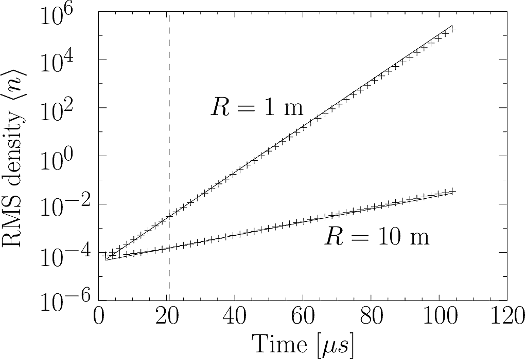
Fig. 2 Interchange instability test. Solid lines are from analytic theory, symbols from BOUT++ simulations, and the RMS density is averaged over \(z\). Vertical dashed line marks the reference point, where analytic and simulation results are set equal#
sod-shock#
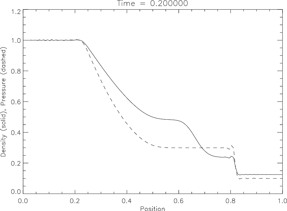
Fig. 3 Sod shock-tube problem for testing shock-handling methods#