Laplacian inversion

A common problem in plasma models is to solve an equation of the form

(3)\[d\nabla^2_\perp x + \frac{1}{c_1}(\nabla_\perp c_2)\cdot\nabla_\perp x + a x = b\]

For example,

\[\nabla_\perp^2 x + a x = b\]

appears in reduced MHD for the vorticity inversion and \(j_{||}\).

Alternative formulations and ways to invert equation (3) can be found in section LaplaceXY and LaplaceXZ

Several implementations of the Laplacian solver are available, which are selected by changing the “type” setting.The currently available implementations are listed in table Table 12.

Table 12 Laplacian implementation types

Name	Description	Requirements
cyclic	Serial/parallel. Gathers boundary rows onto one processor.
petsc	Serial/parallel. Lots of methods, no Boussinesq	PETSc (section PETSc)
petsc3damg	Serial/parallel. Solves full 3D operator (with y-derivatives) with algebraic multigrid.	PETSc (section PETSc)
multigrid	Serial/parallel. Geometric multigrid, no Boussinesq
naulin	Serial/parallel. Iterative treatment of non-Boussinesq terms
serial_tri	Serial only. Thomas algorithm for tridiagonal system.	Lapack (section LAPACK)
serial_band	Serial only. Enables 4th-order accuracy	Lapack (section LAPACK)
spt	Parallel only (NXPE>1). Thomas algorithm.
ipt	Iterative parallel tridiagonal solver. Parallel only, but automatically falls back to Thomas algorithm for NXPE=1.

Usage of the laplacian inversion

In BOUT++, equation (3) can be solved in two ways. The first method Fourier transforms in the \(z\)-direction, whilst the other solves the full two dimensional problem by matrix inversion. The derivation of \(\nabla_\perp^2f\) for a general coordinate system can be found in the Field-aligned coordinates section. What is important, is to note that if \(g_{xy}\) and \(g_{yz}\) are non-zero, BOUT++ neglects the \(y\)-parallel derivatives when using the solvers Laplacian and LaplaceXZ.

By neglecting the \(y\)-derivatives (or if \(g_{xy}=g_{yz}=0\)), one can solve equation (3) \(y\) plane by \(y\) plane.

The first approach utilizes the fact that it is possible to Fourier transform the equation in \(z\) (using some assumptions described in section Numerical implementation), and solve a tridiagonal system for each mode. These inversion problems are band-diagonal (tri-diagonal in the case of 2nd-order differencing) and so inversions can be very efficient: \(O(n_z \log n_z)\) for the FFTs, \(O(n_x)\) for tridiagonal inversion using the Thomas algorithm, where \(n_x\) and \(n_z\) are the number of grid-points in the \(x\) and \(z\) directions respectively.

In the second approach, the full \(2\)-D system is solved. The available solvers for this approach are ‘multigrid’ using a multigrid algorithm; ‘naulin’ using an iterative scheme to correct the FFT-based approach; or ‘petsc’ using KSP linear solvers from the PETSc library (this requires PETSc to be built with BOUT++).

The Laplacian class is defined in invert_laplace.hxx and solves problems formulated like equation (3) To use this class, first create an instance of it:

std::unique_ptr<Laplacian> lap = Laplacian::create();

By default, this will use the options in a section called “laplace”, but can be given a different section as an argument. By default \(d = 1\), \(a = 0\), and \(c_1=c_2=1\). To set the values of these coefficients, there are the setCoefA(), setCoefC1(), setCoefC2(), setCoefC() (which sets both \(c_1\) and \(c_2\) to its argument), and setCoefD() methods:

Field2D a = ...;
lap->setCoefA(a);
lap->setCoefC(0.5);

arguments can be Field2D, Field3D, or BoutReal values. Note that FFT solvers will use only the DC part of Field3D arguments.

Settings for the inversion can be set in the input file under the section laplace (default) or whichever settings section name was specified when the Laplacian class was created. Commonly used settings are listed in tables Table 13 to Table 16.

In particular boundary conditions on the \(x\) boundaries can be set using the and outer_boundary_flags variables, as detailed in table Table 15. Note that DC (‘direct-current’) refers to \(k = 0\) Fourier component, AC (‘alternating-current’) refers to \(k \neq 0\) Fourier components. Non-Fourier solvers use AC options (and ignore DC ones). Multiple boundary conditions can be selected by adding together the required boundary condition flag values together. For example, inner_boundary_flags = 3 will set a Neumann boundary condition on both AC and DC components.

It is pertinent to note here that the boundary in BOUT++ is defined by default to be located half way between the first guard point and first point inside the domain. For example, when a Dirichlet boundary condition is set, using inner_boundary_flags = 0 , 16, or 32, then the first guard point, \(f_{-}\) will be set to \(f_{-} = 2v - f_+\), where \(f_+\) is the first grid point inside the domain, and \(v\) is the value to which the boundary is being set to.

The global_flags, inner_boundary_flags, outer_boundary_flags and flags values can also be set from within the physics module using setGlobalFlags, setInnerBoundaryFlags , setOuterBoundaryFlags and setFlags.

lap->setGlobalFlags(Global_Flags_Value);
lap->setInnerBoundaryFlags(Inner_Flags_Value);
lap->setOuterBoundaryFlags(Outer_Flags_Value);
lap->setFlags(Flags_Value);

Table 13 Laplacian inversion options

Name	Meaning	Default value
type	Which implementation to use. See table Table 12	cyclic
filter	Filter out modes above \((1-\)filter\()\times k_{max}\), if using Fourier solver	0
maxmode	Filter modes with \(n >\)maxmode	MZ/2
all_terms	Include first derivative terms	true
nonuniform	Include corrections for non-uniform meshes (dx not constant)	Same as global non_uniform. See here
global_flags	Sets global inversion options See table Laplace global flags	0
inner_boundary_flags	Sets boundary conditions on inner boundary. See table Laplace boundary flags	0
outer_boundary_flags	Sets boundary conditions on outer boundary. See table Laplace boundary flags	0
flags	DEPRECATED. Sets global solver options and boundary conditions. See Laplace flags or invert_laplace.cxx	0
include_yguards	Perform inversion in \(y\)-boundary guard cells	false

Table 14 Laplacian inversion global_flags values: add the required quantities together.

Flag	Meaning	Code variable
0	No global option set	\(-\)
1	zero DC component (Fourier solvers)	INVERT_ZERO_DC
2	set initial guess to 0 (iterative solvers)	INVERT_START_NEW
4	equivalent to outer_boundary_flags = 128, inner_boundary_flags = 128	INVERT_BOTH_BNDRY_ONE
8	Use 4th order differencing (Apparently not actually implemented anywhere!!!)	INVERT_4TH_ORDER
16	Set constant component (\(k_x = k_z = 0\)) to zero	INVERT_KX_ZERO

Table 15 Laplacian inversion outer_boundary_flags or inner_boundary_flags values: add the required quantities together.

Flag	Meaning	Code variable
0	Dirichlet (Set boundary to 0)	\(-\)
1	Neumann on DC component (set gradient to 0)	INVERT_DC_GRAD
2	Neumann on AC component (set gradient to 0)	INVERT_AC_GRAD
4	Zero or decaying Laplacian on AC components ( \(\frac{\partial^2}{\partial x^2}+k_z^2\) vanishes/decays)	INVERT_AC_LAP
8	Use symmetry to enforce zero value or gradient (redundant for 2nd order now)	INVERT_SYM
16	Set boundary condition to values in boundary guard cells of second argument, x0, of Laplacian::solve(const Field3D &b, const Field3D &x0). May be combined with any combination of 0, 1 and 2, i.e. a Dirichlet or Neumann boundary condition set to values which are \(\neq 0\) or \(f(y)\)	INVERT_SET
32	Set boundary condition to values in boundary guard cells of RHS, b in Laplacian::solve(const Field3D &b, const Field3D &x0). May be combined with any combination of 0, 1 and 2, i.e. a Dirichlet or Neumann boundary condition set to values which are \(\neq 0\) or \(f(y)\)	INVERT_RHS
64	Zero or decaying Laplacian on DC components (\(\frac{\partial^2}{\partial x^2}\) vanishes/decays)	INVERT_DC_LAP
128	Assert that there is only one guard cell in the \(x\)-boundary	INVERT_BNDRY_ONE
256	DC value is set to parallel gradient, \(\nabla_\parallel f\)	INVERT_DC_GRADPAR
512	DC value is set to inverse of parallel gradient \(1/\nabla_\parallel f\)	INVERT_DC_GRADPARINV
1024	Boundary condition for inner ‘boundary’ of cylinder	INVERT_IN_CYLINDER

Table 16 Laplacian inversion flags values (DEPRECATED!): add the required quantities together.

Flag	Meaning
1	Zero-gradient DC on inner (X) boundary. Default is zero-value
2	Zero-gradient AC on inner boundary
4	Zero-gradient DC on outer boundary
8	Zero-gradient AC on outer boundary
16	Zero DC component everywhere
32	Not used currently
64	Set width of boundary to 1 (default is MXG)
128	Use 4\(^{th}\)-order band solver (default is 2\(^{nd}\) order tridiagonal)
256	Attempt to set zero laplacian AC component on inner boundary by combining 2nd and 4th-order differencing at the boundary. Ignored if tridiagonal solver used.
512	Zero laplacian AC on outer boundary
1024	Symmetric boundary condition on inner boundary
2048	Symmetric outer boundary condition

To perform the inversion, there’s the solve method

x = lap->solve(b);

There are also functions compatible with older versions of the BOUT++ code, but these are deprecated:

Field2D a, c, d;
invert_laplace(b, x, flags, &a, &c, &d);

and

x = invert_laplace(b, flags, &a, &c, &d);

The input b and output x are 3D fields, and the coefficients a, c, and d are pointers to 2D fields. To omit any of the three coefficients, set them to NULL.

Numerical implementation

We will here go through the implementation of the laplacian inversion algorithm, as it is performed in BOUT++. We would like to solve the following equation for \(f\)

(4)\[d\nabla_\perp^2f + \frac{1}{c_1}(\nabla_\perp c_2)\cdot\nabla_\perp f + af = b\]

BOUT++ neglects the \(y\)-parallel derivatives if \(g_{xy}\) and \(g_{yz}\) are non-zero when using the solvers Laplacian and LaplaceXZ. For these two solvers, equation (4) becomes (see Field-aligned coordinates for derivation)

(5)\[\begin{split}\, &d (g^{xx} \partial_x^2 + G^x \partial_x + g^{zz} \partial_z^2 + G^z \partial_z + 2g^{xz} \partial_x \partial_z ) f \\ +& \frac{1}{c_1}( {{\boldsymbol{e}}}^x \partial_x + {\boldsymbol{e}}^z \partial_z ) c_2 \cdot ({\boldsymbol{e}}^x \partial_x + {\boldsymbol{e}}^z \partial_z ) f \\ +& af = b\end{split}\]

Using tridiagonal solvers

Since there are no parallel \(y\)-derivatives if \(g_{xy}=g_{yz}=0\) (or if they are neglected), equation (4) will only contain derivatives of \(x\) and \(z\) for the dependent variable. The hope is that the modes in the periodic \(z\) direction will decouple, so that we in the end only have to invert for the \(x\) coordinate.

If the modes decouples when Fourier transforming equation (5), we can use a tridiagonal solver to solve the equation for each Fourier mode.

Using the discrete Fourier transform

\[F(x,y)_{k} = \frac{1}{N}\sum_{Z=0}^{N-1}f(x,y)_{Z}\exp(\frac{-2\pi i k Z}{N})\]

we see that the modes will not decouple if a term consist of a product of two terms which depends on \(z\), as this would give terms like

\[\frac{1}{N}\sum_{Z=0}^{N-1} a(x,y)_Z f(x,y)_Z \exp(\frac{-2\pi i k Z}{N})\]

Thus, in order to use a tridiagonal solver, \(a\), \(c_1\), \(c_2\) and \(d\) cannot be functions of \(z\). Because of this, the \({{\boldsymbol{e}}}^z \partial_z c_2\) term in equation (5) is zero. Thus the tridiagonal solvers solve equations of the form

\[\begin{split}\, &d(x,y) ( g^{xx}(x,y) \partial_x^2 + G^x(x,y) \partial_x + g^{zz}(x,y) \partial_z^2 + G^z(x,y) \partial_z + 2g^{xz}(x,y) \partial_x \partial_z ) f(x,y,z) \\ +& \frac{1}{c_1(x,y)}({{\boldsymbol{e}}}^x \partial_x c_2(x,y) ) \cdot ( {{\boldsymbol{e}}}^x \partial_x + \boldsymbol{e}^z \partial_z) f(x,y,z) \\ +& a(x,y)f(x,y,z) = b(x,y,z)\end{split}\]

after using the discrete Fourier transform (see section Derivatives of the Fourier transform), we get

\[\begin{split}\, &d ( g^{xx} \partial_x^2F_z + G^x \partial_xF_z + g^{zz} [i k]^2F_z + G^z [i k]F_z + 2g^{xz} \partial_x[i k]F_z ) \\ +& \frac{1}{c_1}( {{\boldsymbol{e}}}^x \partial_x c_2 ) \cdot ( {{\boldsymbol{e}}}^x \partial_xF_z + \boldsymbol{e}^z i k F_z) \\ +& aF_z = B_z\end{split}\]

which gives

(6)\[\begin{split}\, &d ( g^{xx} \partial_x^2 + G^x \partial_x - k^2 g^{zz} + i kG^z + i k2g^{xz} \partial_x )F_z \\ +& \frac{1}{c_1} (\partial_x c_2 ) (g^{xx}\partial_xF_z + g^{xz} i k F_z) \\ +& aF_z = B_z\end{split}\]

As nothing in equation (6) couples points in \(y\) together (since we neglected the \(y\)-derivatives if \(g_{xy}\) and \(g_{yz}\) were non-zero) we can solve \(y\)-plane by \(y\)-plane. Also, as the modes are decoupled, we may solve equation (6) \(k\) mode by \(k\) mode in addition to \(y\)-plane by \(y\)-plane.

The second order centred approximation of the first and second derivatives in \(x\) reads

\[\begin{split}\partial_x f &\simeq \frac{-f_{n-1} + f_{n+1}}{2\text{d}x} \\ \partial_x^2 f &\simeq \frac{f_{n-1} - f_{n} + f_{n+1}}{\text{d}x^2}\end{split}\]

This gives

\[\begin{split}\, &d \left( g^{xx} \frac{F_{z,n-1} - 2F_{z,n} + F_{z, n+1}}{\text{d}x^2} + G^x \frac{-F_{z,n-1} + F_{z,n+1}}{2\text{d}x} - k^2 g^{zz}F_{z,n} \right. \\ &\left. \quad + i kG^zF_{z,n} + i k2g^{xz} \frac{-F_{z,n-1} + F_{z,n+1}}{2\text{d}x} \right) \\ +& \frac{1}{c_1} \left( \frac{-c_{2,n-1} + c_{2,n+1}}{2\text{d}x} \right) \left(g^{xx}\frac{-F_{z,n-1} + F_{z,n+1}}{2\text{d}x} + g^{xz} i k F_{z,n} \right) \\ +& aF_{z,n} = B_{z,n}\end{split}\]

collecting point by point

(7)\[\begin{split} &\left( \frac{dg^{xx}}{\text{d}x^2} - \frac{dG^x}{2\text{d}x} - \frac{g^{xx}}{c_{1,n}} \frac{-c_{2,n-1} + c_{2,n+1}}{4\text{d}x^2} - i\frac{d k2g^{xz}}{2\text{d}x} \right) F_{z,n-1} \\ +&\left( - \frac{ dg^{xx} }{\text{d}x^2} - dk^2 g^{zz} + a + idkG^z + i\frac{g^{xz}}{c_{1,n}} \frac{-c_{2,n-1} + c_{2,n+1}}{2\text{d}x}k \right) F_{z,n} \\ +&\left( \frac{dg^{xx}}{\text{d}x^2} + \frac{dG^x}{2\text{d}x} + \frac{g^{xx}}{c_{1,n}} \frac{-c_{2,n-1} + c_{2,n+1}}{4\text{d}x^2} + i\frac{dk2g^{xz}}{2\text{d}x} \right) F_{z, n+1} \\ = B_{z,n}\end{split}\]

We now introduce

\[ \begin{align}\begin{aligned}C_1 &= \frac{dg^{xx}}{\text{d}x^2}\\C_2 &= dg^{zz}\\C_3 &= \frac{2dg^{xz}}{2\text{d}x}\\C_4 &= \frac{dG^x + g^{xx}\frac{-c_{2,n-1} + c_{2,n+1}}{2c_{1,n}\text{d}x}}{2\text{d}x}\\C_5 &= dG^z + \frac{g^{xz}}{c_{1,n}} \frac{-c_{2,n-1} + c_{2,n+1}}{2\text{d}x}\end{aligned}\end{align} \]

which inserted in equation (7) gives

\[( C_1 - C_4 -ikC_3 ) F_{z,n-1} + ( -2C_1 - k^2C_2 +ikC_5 + a ) F_{z,n} + ( C_1 + C_4 + ikC_3 ) F_{z, n+1} = B_{z,n}\]

This can be formulated as the matrix equation

\[AF_z=B_z\]

where the matrix \(A\) is tridiagonal. The boundary conditions are set by setting the first and last rows in \(A\) and \(B_z\).

The tridiagonal solvers previously required \(c_1 = c_2\) in equation (4), but from version 4.3 allow \(c_1 \neq c_2\).

Using PETSc solvers

When using PETSc, all terms of equation (5) are used when inverting to find \(f\). Note that when using PETSc, we do not Fourier decompose in the \(z\)-direction, so it may take substantially longer time to find the solution. As with the tridiagonal solver, the fields are sliced in the \(y\)-direction, and a solution is found for one \(y\) plane at the time.

Before solving, equation (5) is rewritten to the form \(A{{\boldsymbol{x}}} ={{\boldsymbol{b}}}\) (however, the full \(A\) is not expanded in memory). To do this, a row \(i\) in the matrix \(A\) is indexed from bottom left of the two dimensional field \(= (0,0) = 0\) to top right \(= (\texttt{meshx}-1, \texttt{meshz}-1) = \texttt{meshx}\cdot\texttt{meshz}-1\) of the two dimensional field. This is done in such a way so that a row \(i\) in \(A\) increments by \(1\) for an increase of \(1\) in the \(z-\)direction, and by \(\texttt{meshz}\) for an increase of \(1\) in the \(x-\)direction, where the variables \(\texttt{meshx}\) and \(\texttt{meshz}\) represents the highest value of the field in the given direction.

Similarly to equation (7), the discretised version of equation (5) can be written. Doing the same for the full two dimensional case yields:

Second order approximation

\[\begin{split}\; & c_{i,j} f_{i,j} \\ &+ c_{i-1,j-1} f_{i-1,j-1} + c_{i-1,j} f_{i-1,j} \\ &+ c_{i-1,j+1} f_{i-1,j+1} + c_{i,j-1} f_{i,j-1} \\ &+ c_{i,j+1} f_{i,j+1} + c_{i+1,j-1} f_{i+1,j-1} \\ &+ c_{i+1,j} f_{i+1,j} + c_{i+1,j+1} f_{i+1,j+1} \\ =& b_{i,j}\end{split}\]

Fourth order approximation

\[\begin{split}\; & c_{i,j} f_{i,j} \\ &+ c_{i-2,j-2} f_{i-2,j-2} + c_{i-2,j-1} f_{i-2,j-1} \\ &+ c_{i-2,j} f_{i-2,j} + c_{i-2,j+1} f_{i-2,j+1} \\ &+ c_{i-2,j+2} f_{i-2,j+2} + c_{i-1,j-2} f_{i-1,j-2} \\ &+ c_{i-1,j-1} f_{i-1,j-1} + c_{i-1,j} f_{i-1,j} \\ &+ c_{i-1,j+1} f_{i-1,j+1} + c_{i-1,j+2} f_{i-1,j+2} \\ &+ c_{i,j-2} f_{i,j-2} + c_{i,j-1} f_{i,j-1} \\ &+ c_{i,j+1} f_{i,j+1} + c_{i,j+2} f_{i,j+2} \\ &+ c_{i+1,j-2} f_{i+1,j-2} + c_{i+1,j-1} f_{i+1,j-1} \\ &+ c_{i+1,j} f_{i+1,j} + c_{i+1,j+1} f_{i+1,j+1} \\ &+ c_{i+1,j+2} f_{i+1,j+2} + c_{i+2,j-2} f_{i+2,j-2} \\ &+ c_{i+2,j-1} f_{i+2,j-1} + c_{i+2,j} f_{i+2,j} \\ &+ c_{i+2,j+1} f_{i+2,j+1} + c_{i+2,j+2} f_{i+2,j+2} \\ =& b_{i,j}\end{split}\]

To determine the coefficient for each node point, it is convenient to introduce some quantities

\begin{align} &A_0 = a(x,y_{\text{current}},z) &A_1 = dg^{xx}&\\ &A_2 = dg^{zz} &A_3 = 2dg^{xz} \end{align}

In addition, we have:

Second order approximation (5-point stencil)

\[\begin{split}\texttt{ddx\_c} = \frac{\texttt{c2}_{x+1} - \texttt{c2}_{x-1} }{2\texttt{c1}\text{d}x} \\ \texttt{ddz\_c} = \frac{\texttt{c2}_{z+1} - \texttt{c2}_{z-1} }{2\texttt{c1}\text{d}z}\end{split}\]

Fourth order approximation (9-point stencil)

\[\begin{split}\texttt{ddx\_c} = \frac{-\texttt{c2}_{x+2} + 8\texttt{c2}_{x+1} - 8\texttt{c2}_{x-1} + \texttt{c2}_{x-2} }{ 12\texttt{c1}\text{d}x} \\ \texttt{ddz\_c} = \frac{-\texttt{c2}_{z+2} + 8\texttt{c2}_{z+1} - 8\texttt{c2}_{z-1} + \texttt{c2}_{z-2} }{ 12\texttt{c1}\text{d}z}\end{split}\]

This gives

\[\begin{split}A_4 &= dG^x + g^{xx}\texttt{ddx\_c} + g^{xz}\texttt{ddz\_c} \\ A_5 &= dG^z + g^{xz}\texttt{ddx\_c} + g^{xx}\texttt{ddz\_c}\end{split}\]

The coefficients \(c_{i+m,j+n}\) are finally being set according to the appropriate order of discretisation. The coefficients can be found in the file petsc_laplace.cxx.

Example: The 5-point stencil

Let us now consider the 5-point stencil for a mesh with \(3\) inner points in the \(x\)-direction, and \(3\) inner points in the \(z\)-direction. The \(z\) direction will be periodic, and the \(x\) direction will have the boundaries half between the grid-point and the first ghost point (see Fig. 11).

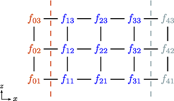
Fig. 11 The mesh: The inner boundary points in \(x\) are coloured in orange, whilst the outer boundary points in \(z\) are coloured gray. Inner points are coloured blue.

Applying the \(5\)-point stencil to point \(f_{22}\) this mesh will result in Fig. 12.

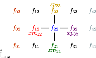
Fig. 12 The mesh with a stencil in point \(f_{22}\): The point under consideration is coloured blue. The point located \(+1\) in \(z\) direction (zp) is coloured yellow and the point located \(-1\) in \(z\) direction (zm) is coloured green. The point located \(+1\) in \(x\) direction (xp) is coloured purple and the point located \(-1\) in \(x\) direction (xm) is coloured red.

We want to solve a problem on the form \(A{{\mathbf{x}}}={{\mathbf{b}}}\). We will order \({{\mathbf{x}}}\) in a row-major order (so that \(z\) is varying faster than \(x\)). Further, we put the inner \(x\) boundary points first in \({{\mathbf{x}}}\), and the outer \(x\) boundary points last in \({{\mathbf{x}}}\). The matrix problem for our mesh can then be written like in Fig. 13.

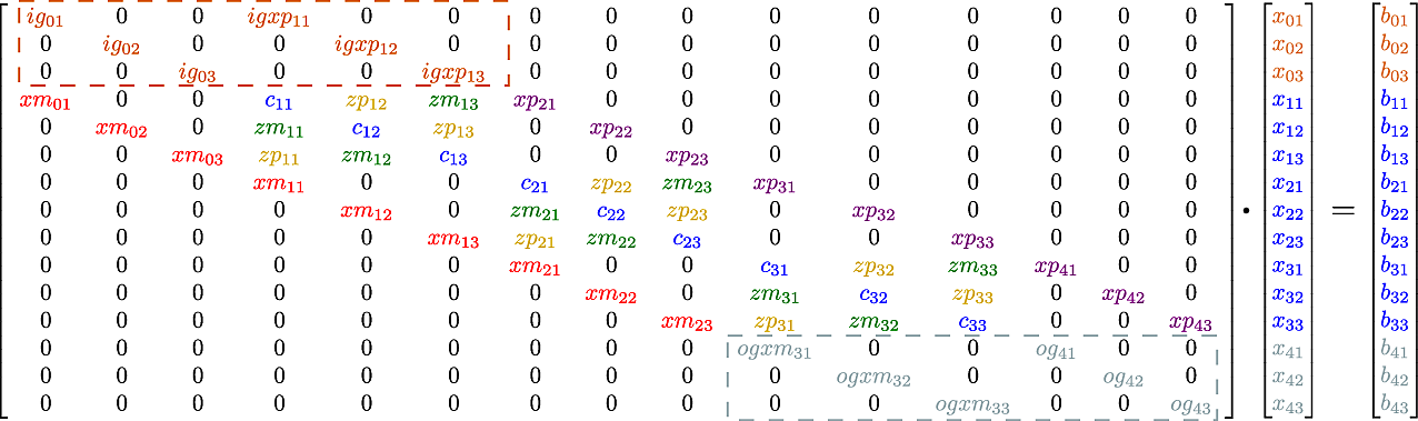
Fig. 13 Matrix problem for our \(3\times3\) mesh: The colors follow that of figure Fig. 11 and Fig. 12. The first index of the elements refers to the \(x\)-position in figure Fig. 11, and the last index of the elements refers to the \(z\)-position in figure Fig. 11. ig refers to “inner ghost point”, og refers to “outer ghost point”, and c refers to the point of consideration. Notice the “wrap-around” in \(z\)-direction when the point of consideration neighbours the first/last \(z\)-index.

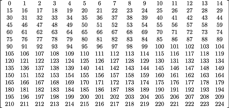
As we are using a row-major implementation, the global indices of the matrix will be as in Fig. 14

Fig. 14 Global indices of the matrix in figure Fig. 13

Implementation internals

The Laplacian inversion code solves the equation:

\[d\nabla^2_\perp x + \frac{1}{c_1}\nabla_\perp c_2\cdot\nabla_\perp x + a x = b\]

where \(x\) and \(b\) are 3D variables, whilst \(a\), \(c_1\), \(c_2\) and \(d\) are 2D variables for the FFT solvers, or 3D variables otherwise. Several different algorithms are implemented for Laplacian inversion, and they differ between serial and parallel versions. Serial inversion can currently either be done using a tridiagonal solver (Thomas algorithm), or a band-solver (allowing \(4^{th}\)-order differencing).

To support multiple implementations, a base class Laplacian is defined in include/invert_laplace.hxx. This defines a set of functions which all implementations must provide:

class Laplacian {
public:
  virtual void setCoefA(const Field2D &val) = 0;
  virtual void setCoefC(const Field2D &val) = 0;
  virtual void setCoefD(const Field2D &val) = 0;

  virtual const FieldPerp solve(const FieldPerp &b) = 0;
}

At minimum, all implementations must provide a way to set coefficients, and a solve function which operates on a single FieldPerp (X-Y) object at once. Several other functions are also virtual, so default code exists but can be overridden by an implementation.

For convenience, the Laplacian base class also defines a function to calculate coefficients in a Tridiagonal matrix:

void tridagCoefs(int jx, int jy, int jz, dcomplex &a, dcomplex &b,
                 dcomplex &c, const Field2D *c1coef = nullptr,
                 const Field2D *c2coef = nullptr,
                 const Field2D *d=nullptr);

For the user of the class, some static functions are defined:

static std::unique_ptr<Laplacian> create(Options *opt = nullptr);
static Laplacian* defaultInstance();

The create function allows new Laplacian implementations to be created, based on options. To use the options in the [laplace] section, just use the default:

std::unique_ptr<Laplacian> lap = Laplacian::create();

The code for the Laplacian base class is in src/invert/laplace/invert_laplace.cxx. The actual creation of new Laplacian implementations is done in the LaplaceFactory class, defined in src/invert/laplace/laplacefactory.cxx. This file includes all the headers for the implementations, and chooses which one to create based on the type setting in the input options. This factory therefore provides a single point of access to the underlying Laplacian inversion implementations.

Each of the implementations is in a subdirectory of src/invert/laplace/impls and is discussed below.

Serial tridiagonal solver

This is the simplest implementation, and is in src/invert/laplace/impls/serial_tri/

Serial band solver

This is band-solver which performs a \(4^{th}\)-order inversion. Currently this is only available when NXPE=1; when more than one processor is used in \(x\), the Laplacian algorithm currently reverts to \(3^{rd}\)-order.

SPT parallel tridiagonal

This is a reference code which performs the same operations as the serial code. To invert a single XZ slice (FieldPerp object), data must pass from the innermost processor (mesh->PE_XIND = 0) to the outermost mesh->PE_XIND = mesh->NXPE-1 and back again.

Some parallelism is achieved by running several inversions simultaneously, so while processor 1 is inverting Y=0, processor 0 is starting on Y=1. This works ok as long as the number of slices to be inverted is greater than the number of X processors (MYSUB > mesh->NXPE). If MYSUB < mesh->NXPE then not all processors can be busy at once, and so efficiency will fall sharply. Fig. 15 shows the useage of 4 processors inverting a set of 3 poloidal slices (i.e. MYSUB=3)

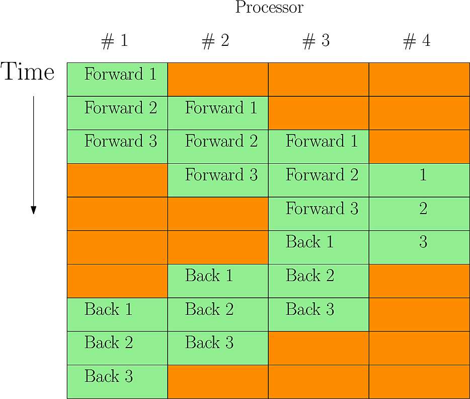
Fig. 15 Parallel Laplacian inversion with MYSUB=3 on 4 processors. Red periods are where a processor is idle - in this case about 40% of the time

Cyclic algorithm

This is now the default solver in both serial and parallel. It is an FFT-based solver using a cyclic reduction algorithm.

Multigrid solver

A solver using a geometric multigrid algorithm was introduced by projects in 2015 and 2016 of CCFE and the EUROfusion HLST.

Naulin solver

This scheme was introduced for BOUT++ by Michael Løiten in the CELMA code and the iterative algorithm is detailed in his thesis [Løiten2017].

The iteration can be under-relaxed (see naulin_laplace.cxx for more details of the implementation). A factor \(0< \text{underrelax\_factor}<=1\) is used, with a value of 1 corresponding to no under-relaxation. If the iteration starts to diverge (the error increases on any step) the underrelax_factor is reduced by a factor of 0.9, and the iteration is restarted from the initial guess. The initial value of underrelax_factor, which underrelax_factor is set to at the beginning of each call to solve can be set by the option initial_underrelax_factor (default is 1.0) in the appropriate section of the input file ([laplace] by default). Reducing the value of initial_underrelax_factor may speed up convergence in some cases. Some statistics from the solver are written to the output files to help in choosing this value. With <i> being the number of the LaplaceNaulin solver, counting in the order they are created in the physics model:

• naulinsolver<i>_mean_underrelax_counts gives the mean number of times underrelax_factor had to be reduced to get the iteration to converge. If this is much above 0, it is probably worth reducing initial_underrelax_factor.

• naulinsolver<i>_mean_its is the mean number of iterations taken to converge. Try to minimise when adjusting initial_underrelax_factor.

[Løiten2017]

Michael Løiten, “Global numerical modeling of magnetized plasma in a linear device”, 2017, https://celma-project.github.io/.

Iterative Parallel Tridiagonal solver

This solver uses a hybrid of multigrid and the Thomas algorithm to invert tridiagonal matrices in parallel. The complexity of the algorithm is O(nx) work and O(log(NXPE)) communications.

The Laplacian is second-order, so to invert it we need two boundary conditions, one at each end of the domain. If we only have one processor, that processor knows both boundary conditions, and we can invert the Laplacian locally using the Thomas algorithm. When the domain is subdivided between two or more processors, we can no longer use the Thomas algorithm, as processors do not know the solution at the subdomain boundaries.

In this hybrid approach, we reduce the original system of equations to a smaller system for solution at the boundaries of each processor’s subdomain. We solve this system in parallel using multigrid. Once the boundary values are known, each processor can find the solution on its subdomain using the Thomas algorithm.

Parameters.

• type = ipt selects this solver.

• rtol and atol are the relative and absolute error tolerances to determine when the residual has converged. The goal of setting these is to minimize the runtime by minimizing the number of iterations required to meet the tolerance. Intuitively we would expect tightening tolerances is bad, as doing so requires more iterations. This is true, but also loosening the tolerances too far can lead to very slowly convergence. Generally, as we scan from large to small tolerances, we start with very slow calculations, then meet some threshold in tolerance where the runtime drops sharply, then see runtime slowly increase again as tolerances tighten further. The run time for all tolerances below this threshold are similar though, and generally it is best to err on the side of tighter tolerances.

• maxits is the maximum number of iterations allowed before the job fails.

• max_cycle is the number of pre and post smoothing operations applied on each multigrid level. The optimal value appears to be max_cycle = 1.

• max_level sets the number of multigrid levels. The optimal value is usually the largest possible value max_level = log2(NXPE) - 2 (see “constraints” below), but sometimes one or two levels less than this can be faster.

• predict_exit. Multigrid convergence rates are very robust. When predict_exit = true, we calculate the convergence rate from early iterations and predict the iteration at which the algorithm will have converged. This allows us to skip convergence checks at most iterations (these checks are expensive as they require global communication). Whether this is advantageous is problem-dependent: it is probably useful at low Z resolution but not at higher Z resolution. This is because the algorithm skips work associated with kz modes which have converged; but if we do not check convergence, we do not know which modes we can skip. Therefore at higher Z resolution we find that reduced communication costs are offset by increased work. predict_exit defaults to false.

Constraints. This method requires that:

• NXPE is a power of 2.

• NXPE > 2^(max_levels+1)

LaplaceXY

Perpendicular Laplacian solver in X-Y.

(8)\[\begin{split}\nabla_\perp f =& \nabla f - \mathbf{b}\left(\mathbf{b}\cdot\nabla\right) \nonumber \\ =& \left(\frac{\partial f}{\partial x} - \frac{g_{xy}}{g_{yy}}\frac{\partial f}{\partial y}\right)\nabla x + \left(\frac{\partial f}{\partial z} - \frac{g_{yz}}{g_{yy}}\frac{\partial f}{\partial y}\right)\nabla z\end{split}\]

In 2D (X-Y), the \(g_{xy}\) component can be dropped since this depends on integrated shear \(I\) which will cancel with the \(g_{xz}\) component. The \(z\) derivative is zero and so this simplifies to

\[\nabla_\perp f = \frac{\partial f}{\partial x}\nabla x - \frac{g_{yz}}{g_{yy}}\frac{\partial f}{\partial y}\nabla z\]

The divergence operator in conservative form is

\[\nabla\cdot\mathbf{A} = \frac{1}{J}\frac{\partial}{\partial u^i}\left(Jg^{ij}A_j\right)\]

and so the perpendicular Laplacian in X-Y is

\[\nabla_\perp^2f = \frac{1}{J}\frac{\partial}{\partial x}\left(Jg^{xx}\frac{\partial f}{\partial x}\right) - \frac{1}{J}\frac{\partial}{\partial y}\left(Jg^{yz}\frac{g_{yz}}{g_{yy}}\frac{\partial f}{\partial y}\right)\]

In field-aligned coordinates, the metrics in the \(y\) derivative term become:

\[g^{yz}\frac{g_{yz}}{g_{yy}} = \frac{B_{tor}^2}{B^2}\frac{1}{h_\theta^2}\]

In the LaplaceXY operator this is implemented in terms of fluxes at cell faces.

\[\frac{1}{J}\frac{\partial}{\partial x}\left(Jg^{xx}\frac{\partial f}{\partial x}\right) \rightarrow \frac{1}{J_i\mathrm{dx_i}}\left[J_{i+1/2}g^{xx}_{i+1/2}\left(\frac{f_{i+1} - f_{i}}{\mathrm{dx}_{i+1/2}}\right) - J_{i-1/2}g^{xx}_{i-1/2}\left(\frac{f_{i} - f_{i-1}}{\mathrm{dx}_{i-1/2}}\right)\right]\]

Notes:

• The ShiftedMetric or FCITransform ParallelTransform must be used (i.e. mesh:paralleltransform:type = shifted or mesh:paralleltransform:type = fci) for this to work, since it assumes that \(g^{xz} = 0\)

• Setting the option pctype = hypre seems to work well, if PETSc has been compiled with the algebraic multigrid library hypre; this can be included by passing the option --download-hypre to PETSc’s configure script.

• LaplaceXY (with the default finite-volume discretisation) has a slightly different convention for passing non-zero boundary values than the Laplacian solvers. LaplaceXY uses the average of the last grid cell and first boundary cell of the initial guess (second argument to solve()) as the value to impose for the boundary condition.

An alternative discretization is available if the option finite_volume = false is set. Then a finite-difference discretization very close to the one used when calling A*Laplace_perp(f) + Grad_perp(A)*Grad_perp(f) + B*f is used. This also supports non-orthogonal grids with \(g^{xy} \neq 0\). The difference is that when \(g^{xy} \neq 0\), Laplace_perp calls D2DXDY(f) which applies a boundary condition to dfdy = DDY(f) before calculating DDX(dfdy) with a slightly different result than the way boundary conditions are applied in LaplaceXY.

• The finite difference implementation of LaplaceXY passes non-zero values for the boundary conditions in the same way as the Laplacian solvers. The value in the first boundary cell of the initial guess (second argument to solve()) is used as the boundary value. (Note that this value is imposed as a boundary condition on the returned solution at a location half way between the last grid cell and first boundary cell.)

LaplaceXZ

This is a Laplacian inversion code in X-Z, similar to the Laplacian solver described in Laplacian inversion. The difference is in the form of the Laplacian equation solved, and the approach used to derive the finite difference formulae. The equation solved is:

\[\nabla\cdot\left( A \nabla_\perp f \right) + Bf = b\]

where \(A\) and \(B\) are coefficients, \(b\) is the known RHS vector (e.g. vorticity), and \(f\) is the unknown quantity to be calculated (e.g. potential), and \(\nabla_\perp f\) is the same as equation ((8)), but with negligible \(y\)-parallel derivatives if \(g_{xy}\), \(g_{yz}\) and \(g_{xz}\) is non-vanishing. The Laplacian is written in conservative form like the LaplaceXY solver, and discretised in terms of fluxes through cell faces.

\[\frac{1}{J}\frac{\partial}{\partial x}\left(J A g^{xx}\frac{\partial f}{\partial x}\right) + \frac{1}{J}\frac{\partial}{\partial z}\left(J A g^{zz}\frac{\partial f}{\partial z}\right) + B f = b\]

The header file is include/bout/invert/laplacexz.hxx. The solver is constructed by using the LaplaceXZ::create() function:

std::unique_ptr<LaplaceXZ> lap = LaplaceXZ::create(mesh);

Note that a pointer to a Mesh object must be given, which for now is the global variable mesh. By default the options section laplacexz is used, so to set the type of solver created, set in the options

[laplacexz]
type = petsc  # Set LaplaceXZ type

or on the command-line laplacexz:type=petsc .

The coefficients must be set using setCoefs . All coefficients must be set at the same time:

lap->setCoefs(1.0, 0.0);

Constants, Field2D or Field3D values can be passed. If the implementation doesn’t support Field3D values then the average over \(z\) will be used as a Field2D value.

To perform the inversion, call the solve function:

Field3D vort = ...;

Field3D phi = lap->solve(vort, 0.0);

The second input to solve is an initial guess for the solution, which can be used by iterative schemes e.g. using PETSc.

Implementations

The currently available implementations are:

• cyclic: This implementation assumes coefficients are constant in \(Z\), and uses FFTs in \(z\) and a complex tridiagonal solver in \(x\) for each \(z\) mode (the CyclicReduction solver). Code in src/invert/laplacexz/impls/cyclic/.

• petsc: This uses the PETSc KSP interface to solve a matrix with coefficients varying in both \(x\) and \(z\). To improve efficiency of direct solves, a different matrix is used for preconditioning. When the coefficients are updated the preconditioner matrix is not usually updated. This means that LU factorisations of the preconditioner can be re-used. Since this factorisation is a large part of the cost of direct solves, this should greatly reduce the run-time.

Test case

The code in examples/test-laplacexz is a simple test case for LaplaceXZ . First it creates a LaplaceXZ object:

std::unique_ptr<LaplaceXZ> inv = LaplaceXZ::create(mesh);

For this test the petsc implementation is the default:

[laplacexz]
type = petsc
ksptype = gmres # Iterative method
pctype  = lu  # Preconditioner

By default the LU preconditioner is used. PETSc’s built-in factorisation only works in serial, so for parallel solves a different package is needed. This is set using:

factor_package = superlu_dist

This setting can be “petsc” for the built-in (serial) code, or one of “superlu”, “superlu_dist”, “mumps”, or “cusparse”.

Then we set the coefficients:

inv->setCoefs(Field3D(1.0),Field3D(0.0));

Note that the scalars need to be cast to fields (Field2D or Field3D) otherwise the call is ambiguous. Using the PETSc command-line flag -mat_view ::ascii_info information on the assembled matrix is printed:

$ mpirun -np 2 ./test-laplacexz -mat_view ::ascii_info
...
Matrix Object: 2 MPI processes
type: mpiaij
rows=1088, cols=1088
total: nonzeros=5248, allocated nonzeros=5248
total number of mallocs used during MatSetValues calls =0
  not using I-node (on process 0) routines
...

which confirms that the matrix element pre-allocation is setting the correct number of non-zero elements, since no additional memory allocation was needed.

A field to invert is created using FieldFactory:

Field3D rhs = FieldFactory::get()->create3D("rhs",
                                            Options::getRoot(),
                                            mesh);

which is currently set to a simple function in the options:

rhs = sin(x - z)

and then the system is solved:

Field3D x = inv->solve(rhs, 0.0);

Using the PETSc command-line flags -ksp_monitor to monitor the iterative solve, and -mat_superlu_dist_statprint to monitor SuperLU_dist we get:

      Nonzeros in L       19984
      Nonzeros in U       19984
      nonzeros in L+U     38880
      nonzeros in LSUB    11900
      NUMfact space (MB) sum(procs):  L\U     0.45    all     0.61
      Total highmark (MB):  All       0.62    Avg     0.31    Max     0.36
      Mat conversion(PETSc->SuperLU_DIST) time (max/min/avg):
                            4.69685e-05 / 4.69685e-05 / 4.69685e-05
      EQUIL time             0.00
      ROWPERM time           0.00
      COLPERM time           0.00
      SYMBFACT time          0.00
      DISTRIBUTE time        0.00
      FACTOR time            0.00
      Factor flops    1.073774e+06    Mflops    222.08
      SOLVE time             0.00
      SOLVE time             0.00
      Solve flops     8.245800e+04    Mflops     28.67
0 KSP Residual norm 5.169560044060e+02
      SOLVE time             0.00
      Solve flops     8.245800e+04    Mflops     60.50
      SOLVE time             0.00
      Solve flops     8.245800e+04    Mflops     49.86
1 KSP Residual norm 1.359142853145e-12

So after the initial setup and factorisation, the system is solved in one iteration using the LU direct solve.

As a test of re-using the preconditioner, the coefficients are then modified:

inv->setCoefs(Field3D(2.0),Field3D(0.1));

and solved again:

      SOLVE time             0.00
      Solve flops     8.245800e+04    Mflops     84.15
0 KSP Residual norm 5.169560044060e+02
      SOLVE time             0.00
      Solve flops     8.245800e+04    Mflops     90.42
      SOLVE time             0.00
      Solve flops     8.245800e+04    Mflops     98.51
1 KSP Residual norm 2.813291076609e+02
      SOLVE time             0.00
      Solve flops     8.245800e+04    Mflops     94.88
2 KSP Residual norm 1.688683980433e+02
      SOLVE time             0.00
      Solve flops     8.245800e+04    Mflops     87.27
3 KSP Residual norm 7.436784980024e+01
      SOLVE time             0.00
      Solve flops     8.245800e+04    Mflops     88.77
4 KSP Residual norm 1.835640800835e+01
      SOLVE time             0.00
      Solve flops     8.245800e+04    Mflops     89.55
5 KSP Residual norm 2.431147365563e+00
      SOLVE time             0.00
      Solve flops     8.245800e+04    Mflops     88.00
6 KSP Residual norm 5.386963293959e-01
      SOLVE time             0.00
      Solve flops     8.245800e+04    Mflops     93.50
7 KSP Residual norm 2.093714782067e-01
      SOLVE time             0.00
      Solve flops     8.245800e+04    Mflops     91.91
8 KSP Residual norm 1.306701698197e-02
      SOLVE time             0.00
      Solve flops     8.245800e+04    Mflops     89.44
9 KSP Residual norm 5.838501185134e-04
      SOLVE time             0.00
      Solve flops     8.245800e+04    Mflops     81.47

Note that this time there is no factorisation step, but the direct solve is still very effective.

Blob2d comparison

The example examples/blob2d-laplacexz is the same as examples/blob2d but with LaplaceXZ rather than Laplacian.

Tests on one processor: Using Boussinesq approximation, so that the matrix elements are not changed, the cyclic solver produces output:

1.000e+02        125       8.28e-01    71.8    8.2    0.4    0.6   18.9
2.000e+02         44       3.00e-01    69.4    8.1    0.4    2.1   20.0

whilst the PETSc solver with LU preconditioner outputs:

1.000e+02        146       1.15e+00    61.9   20.5    0.5    0.9   16.2
2.000e+02         42       3.30e-01    58.2   20.2    0.4    3.7   17.5

so the PETSc direct solver seems to take only slightly longer than the cyclic solver. For comparison, GMRES with Jacobi preconditioning gives:

1.000e+02        130       2.66e+00    24.1   68.3    0.2    0.8    6.6
2.000e+02         78       1.16e+00    33.8   54.9    0.3    1.1    9.9

and with SOR preconditioner:

1.000e+02        124       1.54e+00    38.6   50.2    0.3    0.4   10.5
2.000e+02         45       4.51e-01    46.8   37.8    0.3    1.7   13.4

When the Boussinesq approximation is not used, the PETSc solver with LU preconditioning, re-setting the preconditioner every 100 solves gives:

1.000e+02        142       3.06e+00    23.0   70.7    0.2    0.2    6.0
2.000e+02         41       9.47e-01    21.0   72.1    0.3    0.6    6.1

i.e. around three times slower than the Boussinesq case. When using jacobi preconditioner:

1.000e+02        128       2.59e+00    22.9   70.8    0.2    0.2    5.9
2.000e+02         68       1.18e+00    26.5   64.6    0.2    0.6    8.1

For comparison, the Laplacian solver using the tridiagonal solver as preconditioner gives:

1.000e+02        222       5.70e+00    17.4   77.9    0.1    0.1    4.5
2.000e+02        172       3.84e+00    20.2   74.2    0.2    0.2    5.2

or with Jacobi preconditioner:

1.000e+02        107       3.13e+00    15.8   79.5    0.1    0.2    4.3
2.000e+02        110       2.14e+00    23.5   69.2    0.2    0.3    6.7

The LaplaceXZ solver does not appear to be dramatically faster in serial than the Laplacian solver when the matrix coefficients are modified every solve. When matrix elements are not modified then the solve time is competitive with the tridiagonal solver.

As a test, timing only the setCoefs call for the non-Boussinesq case gives:

1.000e+02        142       1.86e+00    83.3    9.5    0.2    0.3    6.7
2.000e+02         41       5.04e-01    83.1    8.0    0.3    1.2    7.3

so around 9% of the run-time is in setting the coefficients, and the remaining \(\sim 60\)% in the solve itself.