Supported Topologies

BOUT++ can handle any tokamak topology with up to two X-points. Currently, the INGRID and Hypnotoad gridding tools are the tools used to create BOUT++ grids. Hypnotoad can create grids for any of the basic and common topologies while INGRID can create grids for any of the common and complex topologies.

Note

An EQDSK file is needed to create a grid in either of these tools.

Basic Topologies

Basic topologies are used for simpler simulations and don’t need to use the branch cut features. These include:

• “Closed Flux Surface” (CFL): Which encompass the “core” and “SOL” configurations.

• “Open Flux Surface” (OFL): Which encompass the “limiter”, “X-point”, and “slab” configurations.

These don’t require a minimum number of processors to run.

Common Topologies

Single Null (SN)

The most common topology; most tokamaks operate or are able to use this configuration.

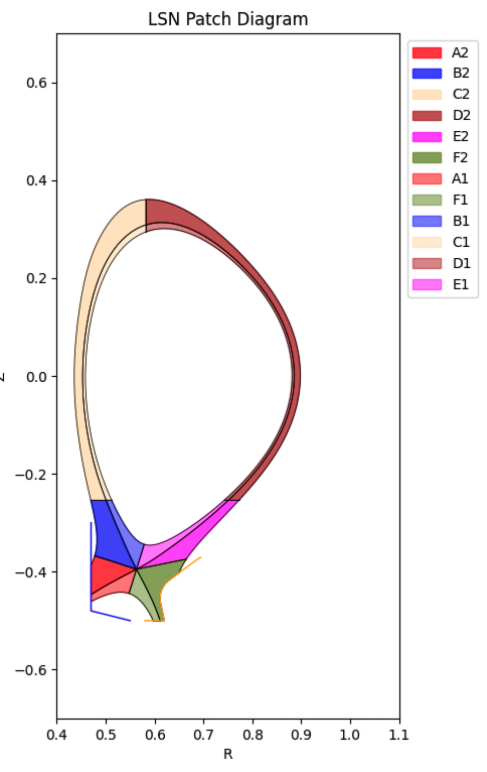
Fig. 21 Single null geometry on the RZ plane generated by INGRID.

The regions that form the building blocks of this topology are:

• 2 “leg” regions which have a boundary in the y direction;

• 1 “core” region which does not have boundaries in y.

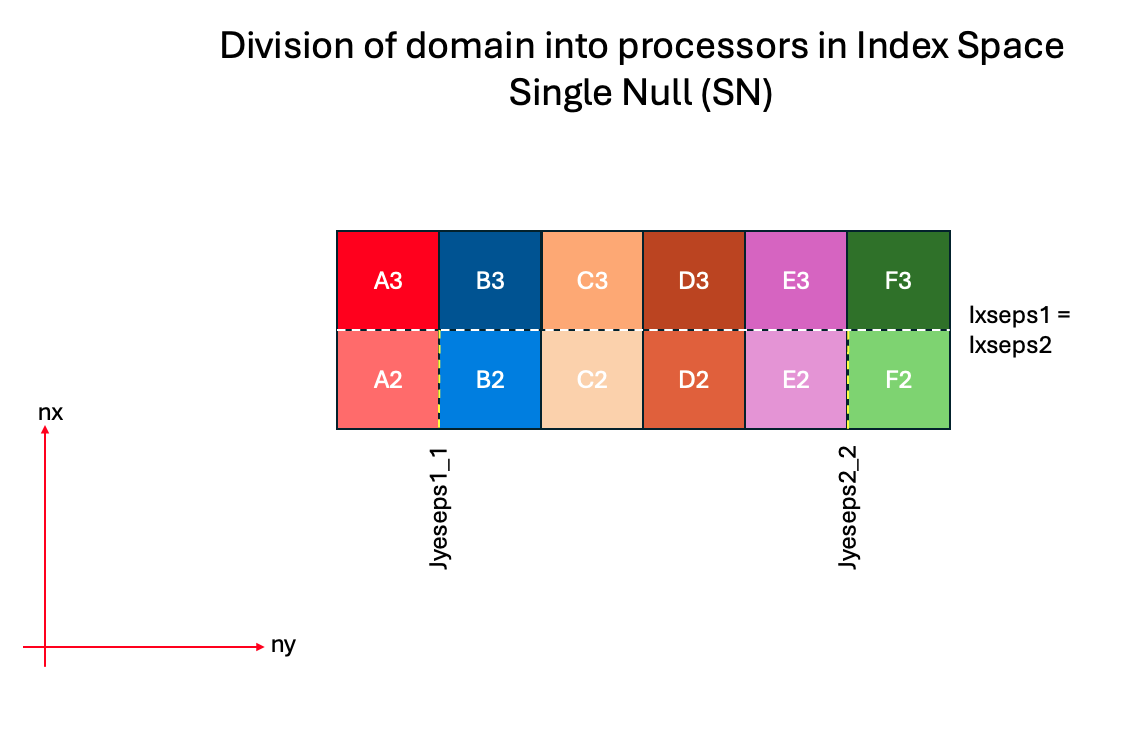
Fig. 22 Division of Single Null configuration into processor layout in index space to compare with the INGRID geometry diagram.

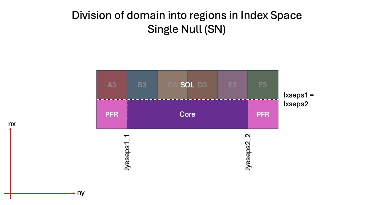
Fig. 23 Single null configuration regions defined by the branch cuts in \(y\).

Even though BOUT++ does not requiere each region to be divided into more processors, using an INGRID grid enables this division and makes it easier to understand the topology.

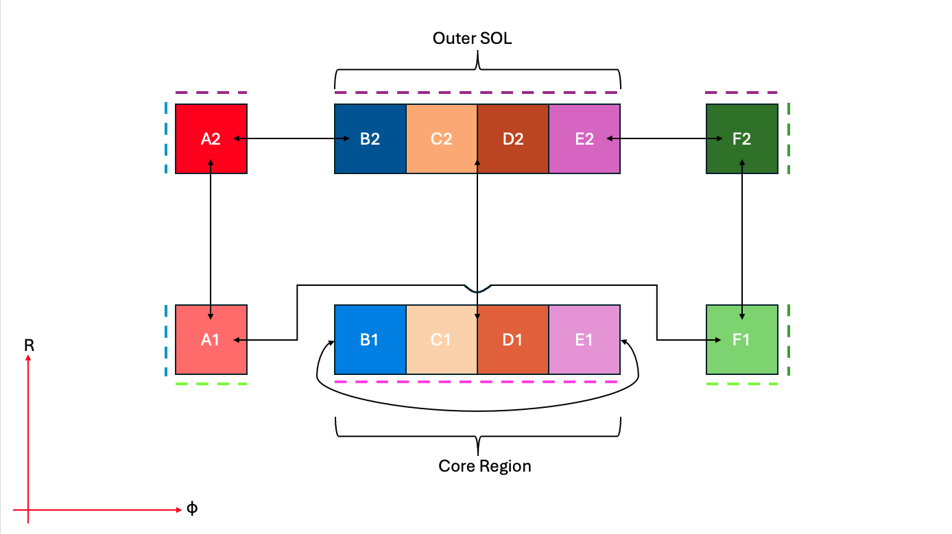
Fig. 24 Single null configuration topology diagram derived from the processor layout.

Connected Double Null (CDN)

The introduction of a secondary divertor on the top of a tokamak is what characterises this configuration. It has a secondary X-point associated with the secondary divertor but the separatrix connects both X-points (ixseps1 == ixseps2). It is an unstable configuration and quite hard to maintain experimentally for a long period of time.

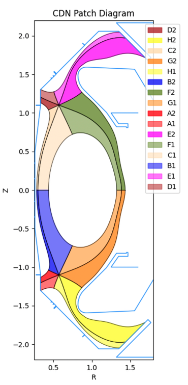
Fig. 25 Connected double null geometry on the RZ plane generated by INGRID.

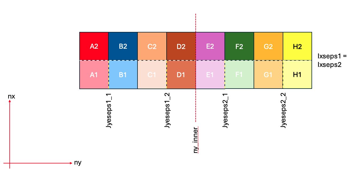
Fig. 26 Division of Connected Double Null configuration into processor layout in index space to compare with the INGRID geometry diagram.

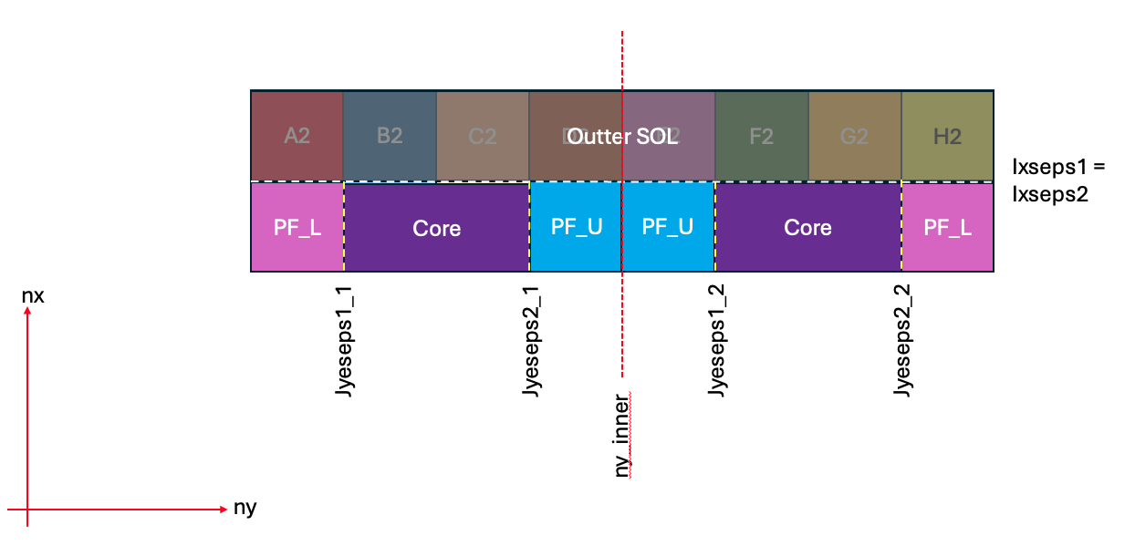
Fig. 27 Connected double null configuration regions defined by the branch cuts in \(y\).

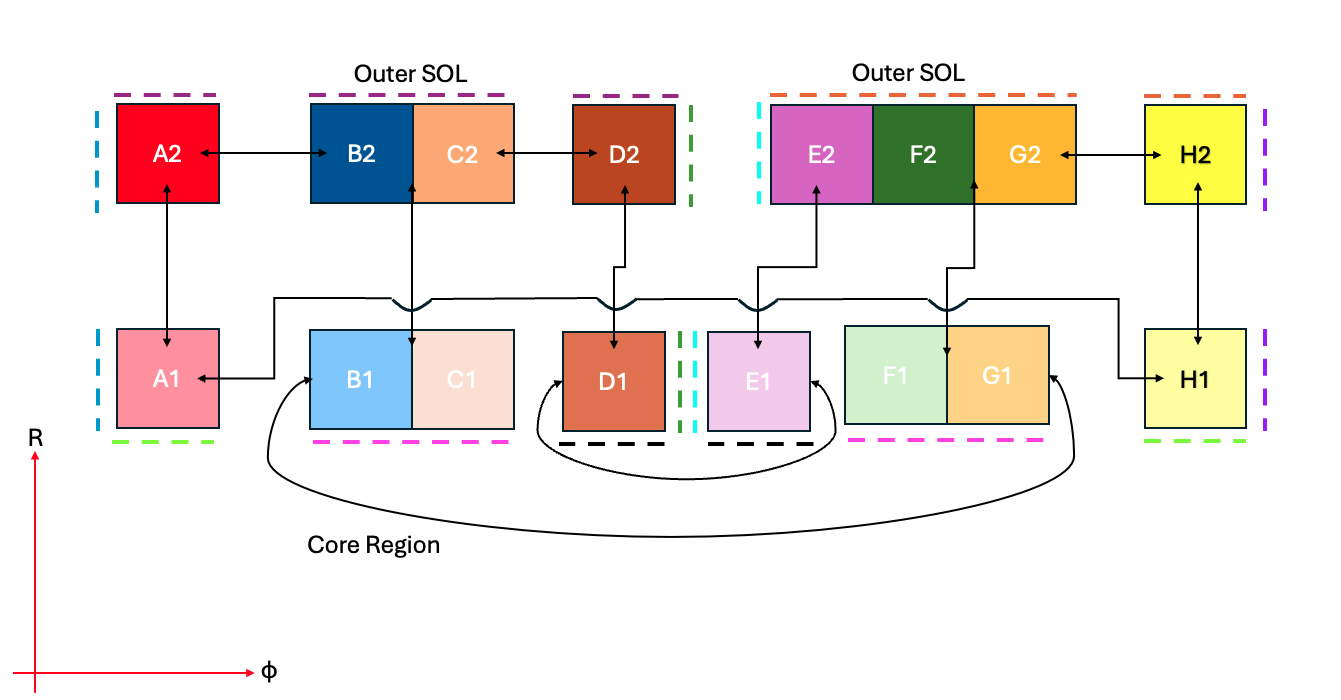
Fig. 28 Connected double null configuration topology diagram derived from the processor layout.

Unconnected Double Null (UDN)

This more realistic configuration has a secondary X-point associated with the secondary divertor but the X-points are not connected, creating a secondary separatrix (ixseps1 != ixseps2). Depending on which separatrix coincides with the start of the inner SOL, it is either an upper or lower UDN. MAST-U is the most famous example of a reactor using the Double Null configurations.

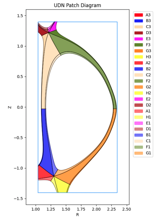
Fig. 29 Unconnected double null geometry on the RZ plane generated by INGRID.

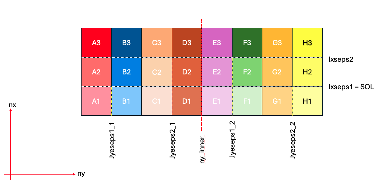
Fig. 30 Division of Unconnected Double Null configuration into processor layout in index space to compare with the INGRID geometry diagram.

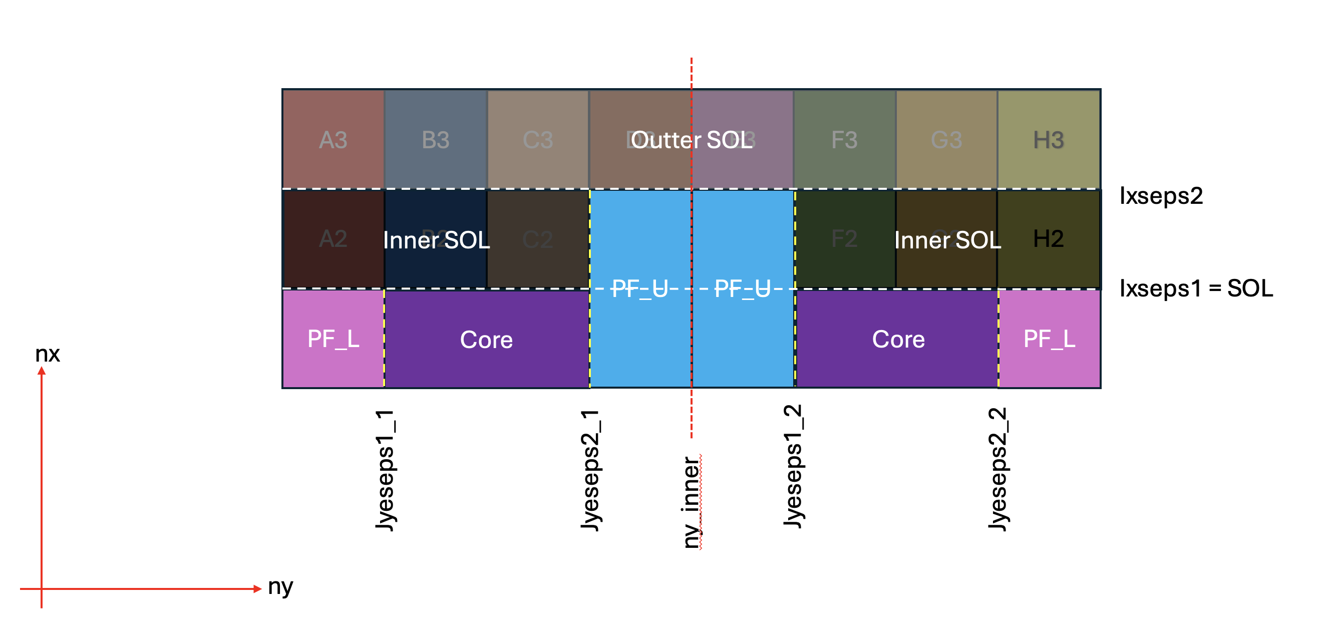
Fig. 31 Unconnected double null configuration regions defined by the branch cuts in \(y\).

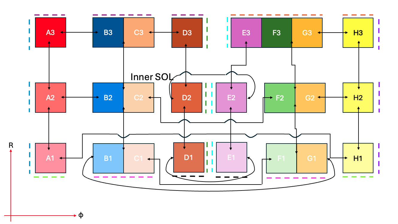
Fig. 32 Unconnected double null configuration topology diagram derived from the processor layout.

Both DN configurations have 2 upper targets defined by ny_inner and ny_inner + 1. The regions that form the building blocks of these topologies are:

• 4 “leg” regions which have a boundary in the y direction;

• 2 “core” regions which do not have boundaries in y.

Complex Topologies

Snowflake (SF)

The snowflake features a secondary X-point close to the primary one. This creates a second-order poloidal field null that branches the separatrix into 4 legs instead of 2. Much like the CDN, the ideal SF is very hard to maintain experimentally, so SF configurations branch into either SF+ or SF-.

Snowflake+ (SF+)

The SF+ configuration has the secondary X-point in the PFR . Unlike the perfect SF, this features an extra central PFR.

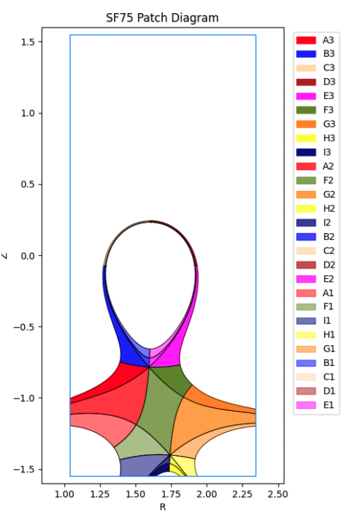
Fig. 33 Snowflake geometry on the RZ plane generated by INGRID.

Snowflake- (SF-)

The SF- configuration has the secondary X-point in the scrape-off layer as opposed to the private flux region. In the case of an “exact” SF-, both X-Points would be at different points on the same flux surface. Usually, SF- configurations have worst heat and particle distributions than the rest of the SF configurations.

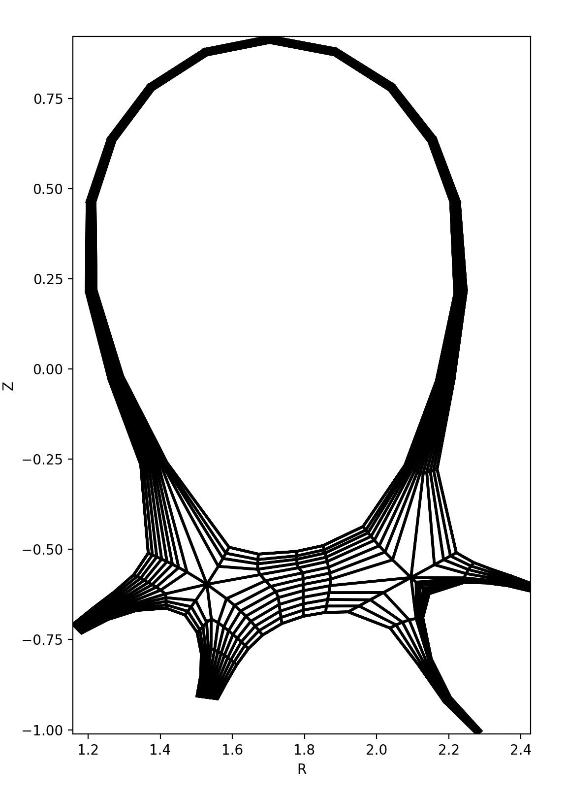
Fig. 34 Snowflake geometry on the RZ plane generated by INGRID.

X-Point Target (XPT)

The X-Point Target configuration has the main separatrix extended a longer distance, the secondary X-point happens far away from the core plasma, and there is no PFR between the East and South East targets. This configuration is especially interesting for studying the effect of detachment and neutral gas injection on the plasma without contaminating the core.

All SF and X-Point Target configurations have 4 targets defined by:

• West on y = 0

• East on y = ny_inner

• South East on y = ny_inner + 1

• South West on y = \(2\pi\)

Topologically, all the SF configurations and the X-Point Target are the same. The regions that form the building blocks of these topologies are:

• 4 “leg” regions which have a boundary in the y direction;

• 1 “core” region which does not have boundaries in y.

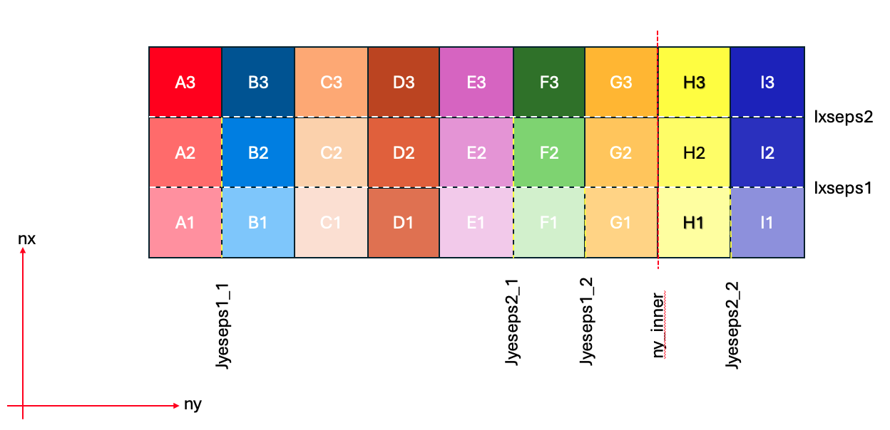
Fig. 35 Division of Snowflake configuration into processor layout in index space to compare with the INGRID geometry diagram.

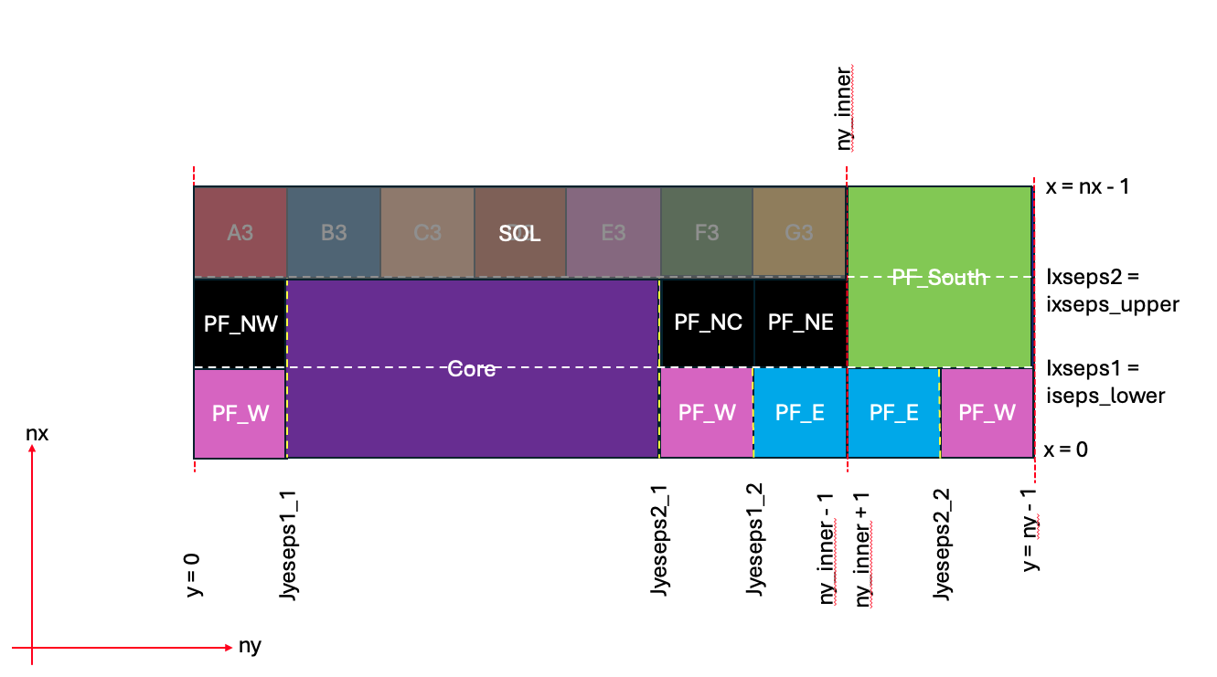
Fig. 36 Snowflake configuration regions defined by the branch cuts in \(y\).

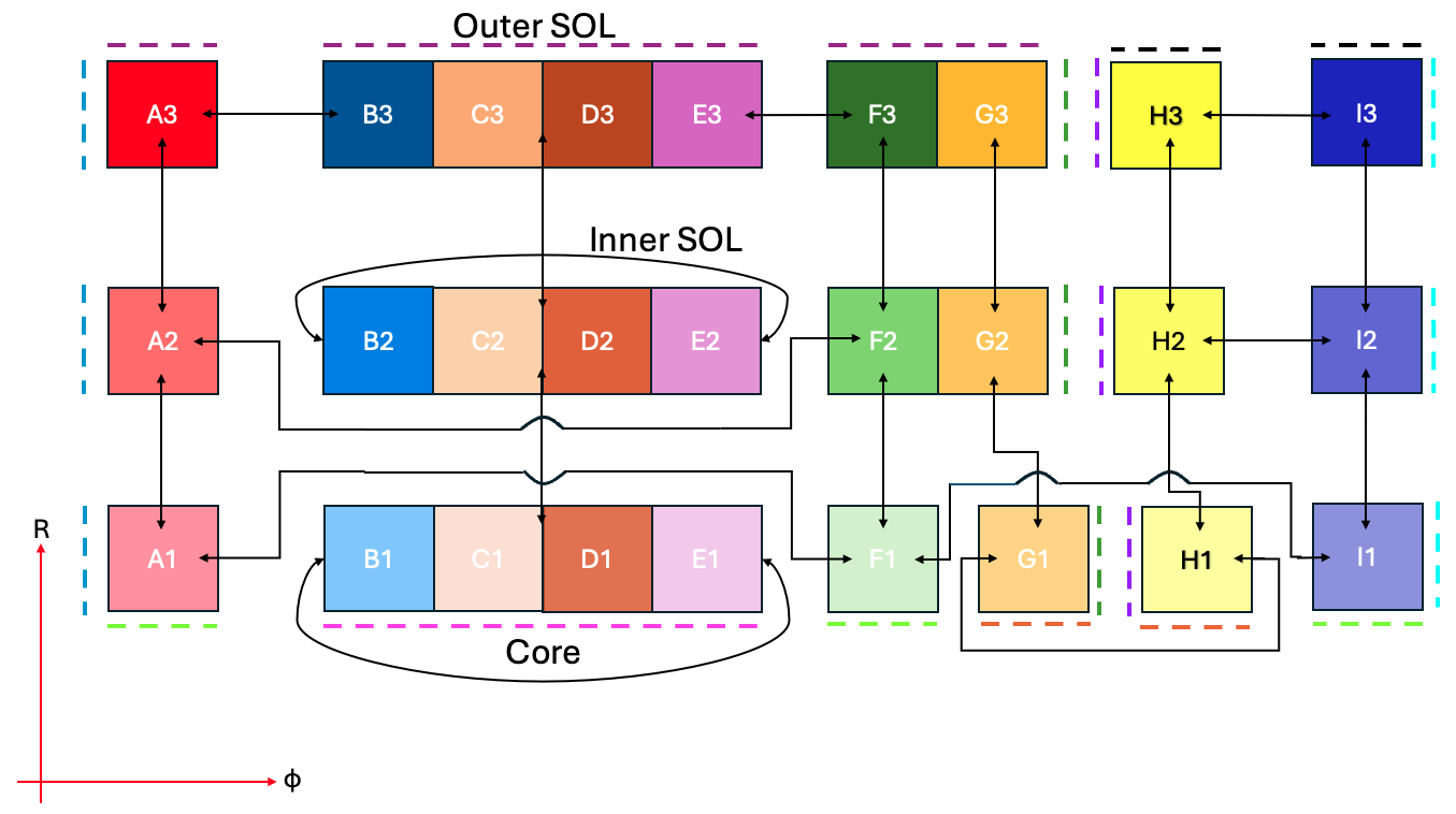
Fig. 37 Snowflake configuration topology diagram derived from the processor layout.