BOUT++ Topology#
Basic#
BOUT++ is designed to work in a variety of tokamak and non-tokamak
geometries, from simple slabs to Snowflake configurations. In order to handle
tokamak geometry BOUT++ contains an internal topology which is built from
regions determined by four branch-cut locations (jyseps*) and two
separatrix locations (ixseps1 and ixseps2). There are some limitations
on these regions that we will discuss below, and some regions may be empty,
all of which enables BOUT++ to describe effectively three types of basic
topologies:
“core”: this type of topology can describe the closed field line regions inside the separatrix of tokamaks or other devices, or idealised geometries like periodic slabs;
“SOL”: these can describe the open field line regions of the scrape-off layer (SOL) outside the separatrix of a tokamak, or linear devices with a target plate at either end;
“limiter”: these topologies have an open field line region and a region where field lines hit a boundary, without an X-point;
“X-point”: these topologies have four separate legs with their own boundaries, and no closed field line region;
The “common” topologies:
“single null”: this type of topology has one X-point with two separate legs, closed and an open field line regions, and a single separatrix;
“connected double null”: these topologies have two X-points with two separate legs each, closed and open field line regions and a single separatrix that connects both X-points;
“disconnected double null”: these are similar to connected double null geometries except that they have two separatrices that do not connect the two X-points. These come in “lower” and “upper” flavours, depending on which X-point is adjacent to the closed field line region.
And all advanced/complex topologies with up to two X-points:
“snowflake”: The SF topologies feature a second order null point created by two X-points close to each other. The ideal SF has a single separatrix and 4 legs, but more realistic configurations can have an extra PFR between the legs. The “snowflake+” and “snowflake-” unlike the perfect SF, feature an extra central PFR and the secondary X-point is located either above or below the primary one, respectively (along the y-direction).
“X-Point Target”: The X-Point Target configuration has the main separatrix extended a longer distance and no PFR between the East and South East targets.
See Supported Topologies for more details on the available topologies.
The regions that form the building blocks of these topologies are:
“leg” regions that have a boundary in the
ydirection;“core” regions that do not have boundaries in
y.
Each of these regions may have additional boundaries in the x direction.
Two important limitations for BOUT++ grids are that a single processor can only belong to one region, and that there must be the same number of points on each processor. The first limitation means that certain topologies require a minimum number of processors. For example, a disconnected double null configuration uses all six regions — therefore the minimum number of processors able to describe this in BOUT++ is six. Having equal numbers of points on each processor can put some restrictions on the resolution of simulations.
The two separatrix locations are ixseps1 and ixseps2, these are the
global indices in the x domain where the first and second separatrices are
located. These values are set either in the grid file or in BOUT.inp.
Considering a Double Null example:
If
ixseps1 == ixseps2then there is a single separatrix representing the boundary between the core region and the SOL region and the grid is a connected double null configuration.If
ixseps1 > ixseps2then there are two separatrices and the inner separatrix isixseps2, so the tokamak is an upper double null.If
ixseps1 < ixseps2then there are two separatrices and the inner separatrix isixseps1, so the tokamak is a lower double null.
In other words: if ixseps1 > ixseps2, then:
f(x <= ixseps1, y, z)will be periodic in they-direction (core),f(ixseps1 < x <= ixseps2, y, z)will have boundary condition inyset by the lowermostydownandyup,f(ixseps2 < x, y, z)will have boundary conditions set by the uppermostydownandyup.
The four branch cut locations, jyseps1_1, jyseps1_2, jyseps2_1, and
jyseps2_2, split the y domain into logical regions defining the SOL, the
PFRs (private flux regions), and the core of the tokamak. If
jyseps1_2 == jyseps2_1 then the grid is a single null configuration,
otherwise it can be any of the more advanced configurations.
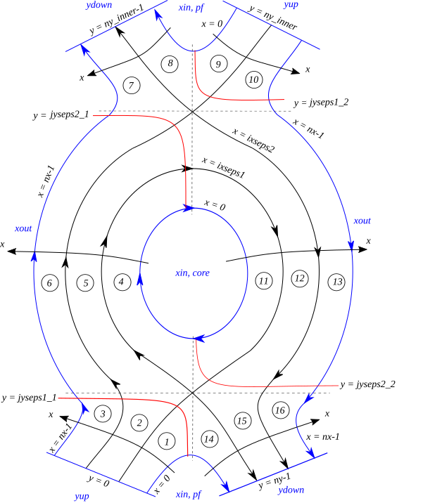
Fig. 18 Deconstruction of a poloidal tokamak cross-section into logical
domains using the parameters ixseps1, ixseps2,
jyseps1_1, jyseps1_2, jyseps2_1, and jyseps2_2. This
configuration is a “disconnected double null” and shows all the
possible regions used in the BOUT++ topology.#
Advanced#
The internal domain in BOUT++ is deconstructed into a series of logically
rectangular sub-domains with boundaries determined by the ixseps and
jyseps parameters. The boundaries coincide with processor boundaries so the
number of grid points within each sub-domain must be an integer multiple of
ny/nypes where ny is the number of grid points in y and nypes
is the number of processors used to split the y domain. Processor communication
across the domain boundaries is then handled internally.
Note
To ensure that each subdomain follows logically, the jyseps indices
must adhere to the following conditions:
jyseps1_1 > -1
jyseps2_1 >= jyseps1_1 + 1
jyseps1_2 >= jyseps2_1
jyseps2_2 >= jyseps1_2
jyseps2_2 <= ny - 1
To ensure that communications work, branch cuts must align with processor boundaries.

Fig. 19 Schematic illustration of domain decomposition and communication in
BOUT++ with ixseps1 = ixseps2#
These branch cuts are used by the getMeshTopology() function to determine
which topology is being used. See Supported Topologies for a
detailed explanation of the available topologies.
Number of targets#
An extra cut in y called ny_inner defines where the physical boundary
in the domain is for topologies with more than 2 targets (any topology more
complex than the single null needs a “discontinuous” \(y\) domain). The position of the extra
cut is what distinguishes any double null configuration from any of the
complex configurations.
Periodic X Domains#
The \(x\) coordinate is usually a radial flux coordinate. In some
simulations it is useful to make this direction periodic, for example flux tube
simulations or the Hasegawa-Wakatani example in
examples/hasegawa-wakatani/hw.cxx. In that example the \(x\) coordinate
is made periodic with the top-level periodicX option:
periodicX = true # Domain is periodic in X

[mesh]

nx = 260  # Note 4 guard cells in X
ny = 1
nz = 256  # Periodic, so no guard cells in Z
Note that some care is needed if the model uses Laplacian inversions, for example to calculate electrostatic potential from vorticity: if both \(x\) and \(z\) coordinates are both periodic then the inversion has no boundary conditions. In that case the Laplacian has a null space and so is singular; an arbitrary constant offset can be added to the potential without changing the vorticity.
The default cyclic solver treats the \(k_z = 0\) (DC) mode as a
special case, setting the average of the potential over the \(x\)-\(z\)
domain to zero. Other solvers may not handle the periodicX case in the same
way.
Implementations#
In BOUT++ each processor has a logically rectangular domain, so any branch cuts needed for X-point geometry must be at processor boundaries.
In the standard “bout” mesh (src/mesh/impls/bout/), the communication is
controlled by the variables
int UDATA_INDEST, UDATA_OUTDEST, UDATA_XSPLIT;
int DDATA_INDEST, DDATA_OUTDEST, DDATA_XSPLIT;
int IDATA_DEST, ODATA_DEST;
These control the behavior of the communications as shown in Fig. 20.
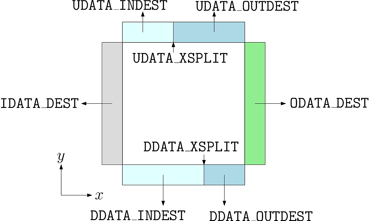
Fig. 20 Communication of guard cells in BOUT++. Boundaries in X have only one neighbour each, but boundaries in Y can be split into two, allowing branch cuts.#
In the Y direction, each boundary region (Up and Down in Y) can be
split into two, with 0 <= x < UDATA_XSPLIT going to processor index
UDATA_INDEST, and UDATA_INDEST <= x < LocalNx going to
UDATA_OUTDEST. Similarly for the Down boundary. Since there are no
branch-cuts in the X direction, there is just one destination for the
Inner and Outer boundaries. In all cases a negative processor
number means that there is a domain boundary so no communication is needed.
The communication control variables are set in the BoutMesh::topology()
function, in src/mesh/impls/bout/boutmesh.cxx. First the function
default_connections() sets the topology to be a rectangle.
To change the topology, the function BoutMesh::set_connection checks that
the requested branch cut is on a processor boundary, and changes the
communications consistently so that communications are two-way and there are no
“dangling” communications.