Arrays, scalar and vector field types#
The classes outlines in red in Fig. 22 are data types currently implemented in BOUT++.
FieldData#
All BOUT++ data types implement a standard interface for accessing their
data, which is then used in communication and file I/O code. This
interface is in src/field/field_data.hxx. The mandatory (pure
virtual) functions are:
bool is3D() const; // True if variable is 3D
with an optional function:
int elementSize() const; // Number of BoutReals in one element
This is only overridden for the Vector2D and Vector3D classes
which essentially have a tuple of (x, y, z) for a single element.
Field#
The two main types are Field2D, and Field3D. Their main functions
are to provide an easy way to manipulate data; they take care of all
memory management, and most looping over grid-points in algebraic
expressions. The 2D field implementation is relatively simple, but
more optimisations are used in the 3D field implementation because
they are much larger (factor of \(\sim 100\)).
To handle time-derivatives, and enable expressions to be written in the following form:
ddt(Ni) = -b0xGrad_dot_Grad(phi, Ni);
fields (and vectors, see below) have a function:
Field3D* timeDeriv();
which returns a pointer to the field holding the time-derivative of this variable. This function ensures that this field is unique using a singleton pattern.
- A
Fieldhas meta-data members, which give: locationis the location of the field values in a grid cell. May be unstaggered,CELL_CENTREor staggered to one of the cell faces,CELL_XLOW,CELL_YLOWorCELL_ZLOW.directionsgives the type of grid that theFieldis defined ondirections.yisYDirectionType::Standardby default, but can beYDirectionType::Alignedif theFieldhas been transformed from an ‘orthogonal’ to a ‘field-aligned’ coordinate system.directions.zisZDirectionType::Standardby default, but can beZDirectionType::Averageif theFieldrepresents a quantity that is averaged or constant in the z-direction (i.e. is aField2D).
The meta-data members are written to the output files as attributes of the variables.
To create a new Field with meta-data, plus Mesh and Coordinates
pointers copied from another one, and data allocated (so that the Field is
ready to use) but not initialized, use the function emptyFrom(const T& f)
which can act on Field3D, Field2D or FieldPerp. This is often used for
example to create a result variable that will be returned from a function
from the Field which is given as input, e.g.
Field3D exampleFunction(const Field3D& f) {
  Field3D result{emptyFrom(f)};
  ...
  < do things to calculate result >
  ...
  return result;
}
To zero-initialise the Field as well, use zeroFrom in place of
emptyFrom. If a few of the meta-data members need to be changed, you can
also chain setter methods to a Field. At the moment the available methods are
setLocation(CELL_LOC), setDirectionY(YDirectionType) and
setDirectionZ(ZDirectionType); also setIndex(int) for FieldPerp. For
example, to set the location of result explicitly you could use
Field3D result{emptyFrom(f).setLocation(CELL_YLOW)};
Vector#
Vector classes build on the field classes, just using a field to represent each component.
To handle time-derivatives of vectors, some care is needed to ensure that the time-derivative of each vector component points to the same field as the corresponding component of the time-derivative of the vector:
ddt(v.x) = ddt(v).x
dcomplex#
Several parts of the BOUT++ code involve FFTs and are therefore much
easier to write using complex numbers. Unfortunately, the C++ complex
library also tries to define a real type, which is already defined
by PVODE. Several work-arounds were tried, some of which worked on some
systems, but it was easier in the end to just implement a new class
dcomplex to handle complex numbers.
Memory management#
This code has been thoroughly tested/debugged, and should only be altered with great care, since just about every other part of BOUT++ depends on this code working correctly. Two optimisations used in the data objects to speed up code execution are memory recycling, which eliminates allocation and freeing of memory; and copy-on-change, which minimises unnecessary copying of data.
Both of these optimisations are done “behind the scenes”, hidden from the remainder of the code, and are illustrated in Fig. 23:
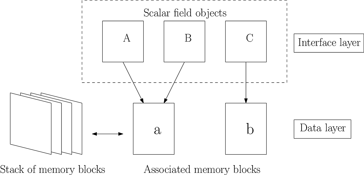
Fig. 23 Memory handling in BOUT++. Memory allocation and freeing is
eliminated by recycling memory blocks, and assignments without
changes (A = B) do not result in copying data, only pointers to
the data. Both these optimisations are handled internally, and are
invisible to the programmer.#
The objects (A,B,C) accessed by the user in operations discussed in the previous section act as an interface to underlying data (a,b). Memory recycling can be used because all the scalar fields are the same size (and vector fields are implemented as a set of 3 scalar fields). Each class implements a global stack of available memory blocks. When an object is assigned a value, it attempts to grab one of these memory blocks, and if none are available then a new block is allocated. When an object is destroyed, its memory block is not freed, but is put onto the stack. Since the evaluation of the time-derivatives involves the same set of operations each time, this system means that memory is only allocated the first time the time-derivatives are calculated, after which the same memory blocks are re-used. This eliminates the often slow system calls needed to allocate and free memory, replacing them with fast pointer manipulation.
Copy-on-change (reference counting) further reduces memory useage and
unnecessary copying of data. When one field is set equal to another
(e.g. Field3D A = B in Fig. 23), no data is copied, only
the reference to the underlying data (in this case both A and B point to
data block a). Only when one of these objects is modified is a second
memory block used to store the different value. This is particularly
useful when returning objects from a routine. Usually this would involve
copying data from one object to another, and then destroying the
original copy. Using reference counting this copying is eliminated.
Global field gather / scatter#
In BOUT++ each processor performs calculations on a sub-set of the
mesh, and communicates with other processors primarily through
exchange of guard cells (the mesh->commmunicate function). If you
need to gather data from the entire mesh onto a single processor, then
this can be done using either 2D or 3D GlobalFields .
First include the header file
#include <bout/globalfield.hxx>
which defines both GlobalField2D and GlobalField3D . To create a
3D global field, pass it the mesh pointer:
GlobalField3D g3d(mesh);
By default all data will be gathered onto processor 0. To change this, specify which processor the data should go to as the second input
GlobalField3D g3d(mesh, processor);
Gather and scatter methods are defined:
Field3D localData;
// Set local data to some value

g3d.gather(localData);  // Gathers all data onto one processor

localData = g3d.scatter(); // Scatter data back
Note: Boundary guard cells are not handled by the scatter step, as this would mean handling branch-cuts etc. To obtain valid data in the guard and Y boundary cells, you will need to communicate and set Y boundaries.
Note: Gather and Scatter are global operations, so all processors must call these functions.
Once data has been gathered, it can be used on one processor. To check
if the data is available, call the method dataIsLocal(), which will
return true only on one processor
if(g3d.dataIsLocal()) {
  // Data is available on this processor

}
The sizes of the global array are available through xSize(),
ySize() and zSize() methods. The data itself can be accessed
indirectly using (x,y,z) operators:
for(int x=0; x<g3d.xSize(); x++)
  for(int y=0; y<g3d.ySize(); y++)
    for(int z=0; z<g3d.zSize(); z++)
      output.write("Value at (%d,%d,%d) is %e\n",
      x,y,z,
      g3d(x,y,z) );
or by getting a pointer to the underlying data, which is stored as a 1D array:
BoutReal *data = g3d.getData();
nx = g3d.xSize();
ny = g3d.ySize();
nz = g3d.zSize();

data[x*ny*nz + y*nz + z]; // Value at g3d(x,y,z)
See the example examples/test-globalfield for more examples.
Iterating over fields#
The recommended way to iterate over a field is to use the BOUT_FOR
macro:
Field3D f(0.0);
BOUT_FOR(i, f.getMesh()->getRegion3D("RGN_ALL")) {
   f[i] = a[i] + b[i];
}
This expands into two nested loops, which have been designed to OpenMP parallelise and vectorise. Some tuning of this is possible, see below for details. It replaces the C-style triple-nested loop:
Field3D f(0.0);
for (int i = mesh->xstart; i < mesh->xend; ++i) {
  for (int j = mesh->ystart; j < mesh->yend; ++j) {
    for (int k = 0; k < mesh->LocalNz; ++k) {
      f(i,j,k) = a(i,j,k) + b(i,j,k)
    }
  }
}
The region to iterate over can be over Field2D, Field3D, or
FieldPerp domains, obtained by calling functions on Mesh:
getRegion2D("name"), getRegion3D("name") and
getRegionPerp("name") respectively. Currently the available regions include:
RGN_ALL, which is the whole mesh;RGN_NOBNDRY, which skips all boundaries and guard cells;RGN_GUARDS, which is only guard cells, both boundary and communication cells;RGN_NOX, which skips the x boundaries and guard cellsRGN_NOY, which skips the y boundaries and guard cells
New regions can be created and modified, see section below.
A standard C++ range for loop can also be used, but this is unlikely to OpenMP parallelise or vectorise:
Field3D f(0.0);
for (auto i : f) {
   f[i] = a[i] + b[i];
}
If you wish to vectorise but can’t use OpenMP then there is a serial verion of the macro:
BoutReal max=0.;
BOUT_FOR_SERIAL(i, region) {
  max = f[i] > max ? f[i] : max;
}
For loops inside parallel regions, there is BOUT_FOR_INNER:
Field3D f(0.0);
BOUT_OMP_PERF(parallel) {
  BOUT_FOR_INNER(i, f.getMesh()->getRegion3D("RGN_ALL")) {
     f[i] = a[i] + b[i];
  }
  ...
}
If a more general OpenMP directive is needed, there is
BOUT_FOR_OMP:
BoutReal result=0.;
BOUT_FOR_OMP(i, region, parallel for reduction(max:result)) {
  result = f[i] > result ? f[i] : result;
}
The iterator provides access to the x, y, z indices:
Field3D f(0.0);
BOUT_FOR(i, f.getMesh()->getRegion3D("RGN_ALL")) {
  f[i] = i.x() + i.y() + i.z();
}
Note that calculating these indices involves some overhead: The iterator uses a single index internally, so integer division and modulo operators are needed to calculate individual indices.
To perform finite difference or similar operators, index offsets can be calculated:
Field3D f = ...;
Field3D g(0.0);
BOUT_FOR(i, f.getMesh()->getRegion3D("RGN_NOBNDRY")) {
  g[i] = f[i.xp()] - f[i.xm()];
}
The xp() function by default produces an offset of +1 in X, xm()
an offset of -1 in the X direction. These functions can also
be given an optional step size argument e.g. xp(2) produces an
offset of +2 in the X direction. There are also xpp(),
which produces an offset of +2, xmm() an offset of -2, and
similar functions exist for Y and Z directions. For other
offsets there is a function offset(x,y,z) so that
i.offset(1,0,1) is the index at (x+1,y,z+1).
Note that by default no bounds checking is performed. If the checking
level is increased to 3 or above then bounds checks will be
performed. This will have a significant (bad) impact on performance, so is
just for debugging purposes. Configure with -DCHECK=3
option to do this.
Tuning BOUT_FOR loops#
The BOUT_FOR macros use two nested loops: The outer loop is OpenMP
parallelised, and iterates over contiguous blocks:
BOUT_OMP_PERF(parallel for schedule(guided))
for (auto block = region.getBlocks().cbegin();
     block < region.getBlocks().cend();
     ++block)
  for (auto index = block->first; index < block->second; ++index)
The inner loop iterates over a contiguous range of indices, which enables it to be vectorised by GCC and Intel compilers.
In order to OpenMP parallelise, there must be enough blocks to
keep all threads busy. In order to vectorise, each of these blocks
must be larger than the processor vector width, preferably several
times larger. This can be tuned by setting the maximum block size,
set at runtime using the mesh:maxregionblocksize option on the
command line or in the BOUT.inp input file:
[mesh]
maxregionblocksize = 64
The default value is set in include/bout/region.hxx:
#define MAXREGIONBLOCKSIZE 64
By default a value of 64 is used, since this has been found to give
good performance on typical x86_64 hardware. Some simple diagnostics
are printed at the start of the BOUT++ output which may help. For
example the blob2d example prints:
Registered region 3D RGN_ALL:
      Total blocks : 1040, min(count)/max(count) : 64 (1040)/ 64 (1040), Max imbalance : 1, Small block count : 0
In this case all blocks are the same size, so the Max imbalance
(ratio of maximum to minimum block size) is 1. The Small block
count is currently defined as the number of blocks with a size less
than half the maximum block size. Ideally all blocks should be a
similar size, so that work is evenly balanced between threads.
Creating new regions#
Regions can be combined in various ways to create new regions. Adding regions together results in a region containing the union of the indices in both regions:
auto region = mesh->getRegion2D("RGN_NOBNDRY") + mesh->getRegion2D("RGN_BNDRY");
This new region could contain duplicated indices, so if unique points
are required then the unique function can be used:
auto region = unique(mesh->getRegion2D("RGN_NOBNDRY") + mesh->getRegion2D("RGN_BNDRY"));
Currently the implementation of unique also sorts the indices, but
if this changes in future there is also a sort function which
ensures that indices are in ascending order. This can help improve the
division into blocks of contiguous indices.
Points can also be removed from regions using the mask
function. This removes all points in the region which are
in the mask (i.e. set subtraction):
auto region = mesh->getRegion2D("RGN_ALL").mask(mesh->getRegion2D("RGN_GUARDS"));
or:
auto region = mask(mesh->getRegion2D("RGN_ALL"), mesh->getRegion2D("RGN_GUARDS"));
The above example would produce a region containing all the indices in
RGN_ALL which are not in RGN_GUARDS.
Currently creating new regions is a relatively slow process, so creating new regions should be done in the initialisation stages rather than in inner loops. Some of this overhead could be reduced with caching, but is not done yet.
One way to improve the performance, and make use of custom regions more convenient, is to register a new region in the mesh:
mesh->addRegion3D("Custom region",
                   mesh->getRegion3D("RGN_NOBNDRY") + mesh->getRegion3D("RGN_BNDRY"));
It is advisable, though not required, to register both 2D and 3D regions of the same name.
In the current implementation overwriting a region, by attempting to
add a region which already exists, is not allowed, and will result in
a BoutException being thrown. This restriction may be removed in
future.
Iterating over ranges#
The boundary of a processor’s domain may consist of a set of disjoint
ranges, so the mesh needs a clean way to tell any code which depends
on the boundary how to iterate over it. The RangeIterator class in
include/bout/sys/range.hxx and src/sys/range.cxx provides
this.
RangeIterator can represent a single continuous range, constructed by passing the minimum and maximum values.
RangeIterator it(1,4);  // Range includes both end points
for(it.first(); !it.isDone(); it.next())
  cout << it.ind; // Prints 1234
A more canonical C++ style is also supported, using overloaded ++,
*, and != operators:
for(it.first(); it != RangeIterator::end(); it++)
  cout << *it; // Prints 1234
where it++ is the same as it.next(), and *it the same as
it.ind.
To iterate over several ranges, RangeIterator can be constructed
with the next range as an argument:
RangeIterator it(1,4, RangeIterator(6,9));
for(it.first(); it != RangeIterator::end(); it++)
  cout << *it; // Prints 12346789
and these can be chained together to an arbitrary depth.
To support statements like:
for(RangeIterator it = mesh->iterateBndryLowerY(); !it.isDone(); it++)
  ...
the initial call to first() is optional, and everything is
initialised in the constructor.
Field2D/Field3D Arithmetic Operators#
The arithmetic operators (+, -, /, *) for Field2D
and Field3D are generated automatically using the Jinja
templating system. This requires Python 3 (2.7 may work, but only 3 is
supported).
Because this is fairly low-level code, and we don’t expect it to
change very much, the generated code is kept in the git
repository. This has the benefit that Python and Jinja are not needed
to build BOUT++, only to change the Field operator code.
Warning
You should not modify the generated code directly. Instead, modify the template and re-generate the code. If you commit changes to the template and/or driver, make sure to re-generate the code and commit it as well
The Jinja template is in src/field/gen_fieldops.jinja, and the
driver is src/field/gen_fieldops.py. The driver loops over every
combination of BoutReal, Field2D, Field3D (collectively just
“fields” here) with the arithmetic operators, and uses the template to
generate the appropriate code. There is some logic in the template to
handle certain combinations of the input fields: for example, for the
binary infix operators, only check the two arguments are on identical
meshes if neither is BoutReal.
To install Jinja:
$ pip3 install --user Jinja2
To re-generate the code, there is a make target for
gen_fieldops.cxx in src/field/makefile. This also tries to
apply clang-format in order to keep to a consistent code style.
Note
clang-format is bundled with clang. This should be
available through your system package manager. If you do not
have sufficient privileges on your system, you can install
it from the source clang. One of the BOUT++ maintainers
can help apply it for you too.